Deep Learning | One Page Knowledge

Source

The material based mostly on the free deep learning course and library fast.ai (from 2017)

https://course.fast.ai/index.html

GPU Servers

This is a short list of GPU Servers that can be used for fast.ai.

Server	Free	Description	Limitation
Google Colab	Yes	Free notebook for use (required setup a GPU)	12 continuus hours per session
Kaggle Notebook	Yes	Free kaggle notebook more	60 continuus minutes per session.
Paperspace	No	Pay as you go consoles to run machines
Microsoft Azure ML	No/200$ for start	Free 200$ for machines that can have GPU inside
Google Cloud	No/300$ for start	Free Tier to use $300 dolars more
Amazon AWS	No	Free Tier doesn’t have GPU machines.

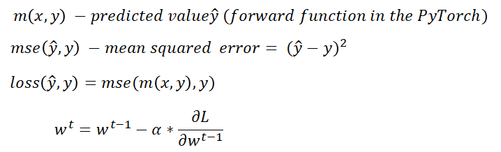
Artificial Neural Network more

Artificial Neural Network (ANN) is an paradigm for the deep learning method based on how the natural nervous system works. They can be used in the ImageRecognition, SpeechRecognition, natural language processing, desease recognition etc…

The simplest architecture of the Artifical Neural Network is a Single-layer Perceptron that was introduced in the 1957 by Frank Rosenblatt. wiki

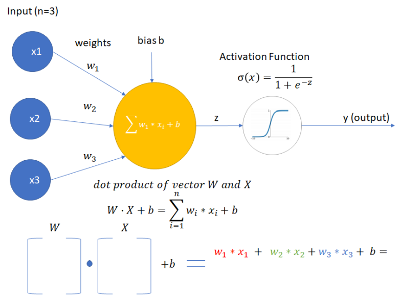
Single Layer Perceptron

This architecture contains:

Input x as a vector
Weights for each x input (w)
bias (b)
and Activation function that on output has been activated or not (0 or 1)

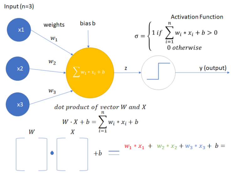σ = 1

When Use?

Can only classify linearly separable cases with the binary output (0 or 1)
Single Layer perceptron cannot solve non-linear problem.
Not used in modern Deep Learning architecture

Modern Neural Network

Modern Neural Networks has something more than only one layer. In previous architecture, you wouldn’t find any better calculation than some simple linear functions. To create more complicated functions we need hidden layers. With this first input goes to the activation function in the first layer, and the following output if the hidden layer can go to the next layer with the activation function or to the final output. More dense Neural Network gives us the opportunity to define more parameters on weights and biases in the network and next recognise more complicated tasks. Each layer can have some special functions. For example in the image recognition first layer is used to extract features (like edges) on the image.

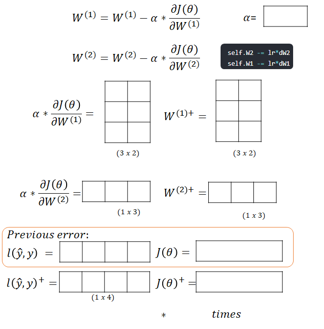
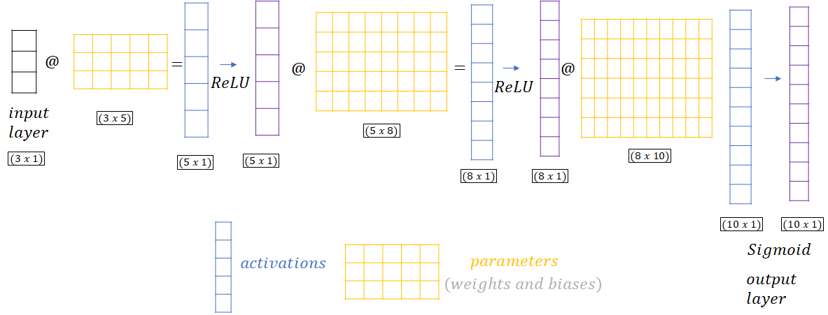
For example, we define a neural network with one hidden layer with three neurons, two input values, and one output. For the moment we don’t set our activation function yet.

1547391156214

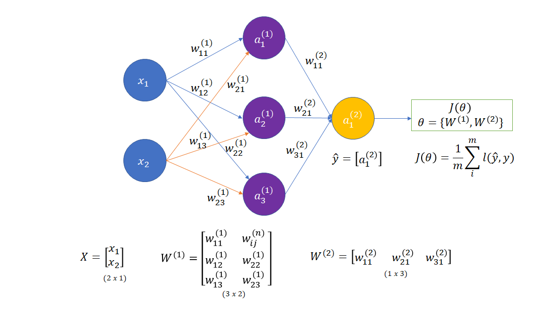
Let’s explain all parameters defined in the network:

Value	Description
	Number of the examples.
	Input on the i position. Sometimes it shows as a zero activation layer.
	Input vector. The size of the input vector is (input_layer x m) . Where m is a number of examples (In this example 1).
	the weight on the layer n, from the input from the previous layer position (i) to the activation layer position (j)
	The matrix on the layer n. The size of the matrix is (current_layer x previous_layer). In the example (3 x 2)
	The Z value on the layer (n). The product on output from the previous layer (or input) and weights on the current layer. The size of the matrix is (current_layer x m)
	The value on the activation function on the layer n and position j. Activation on the last layer is the output on the neural network:
	Activation matrix on the layer (n). The size is the same as
	Set of parameters of the model. In the example two matricies:
	Loss function on the one example.
	Cost function on all examples in the one batch. (Very often show as C or E)

import torch
import torch.nn as nn
import torch.nn.functional as F

class Neural_Network(nn.Module):
    def __init__(self, inputSize = 2, outputSize = 1, hiddenSize = 3 ):
        super(Neural_Network, self).__init__()
        # parameters
        self.inputSize = inputSize
        self.outputSize = outputSize
        self.hiddenSize = hiddenSize
        
        # weights
        #self.W1 = torch.randn(self.hiddenSize, self.inputSize) # 3 X 2 tensor
        #self.W2 = torch.randn(self.outputSize, self.hiddenSize) # 1 X 3 tensor
        self.W1 = torch.tensor([[0.5,0.5],[0.6,0.7],[0.6,0.7]])
        self.W2 = torch.tensor([[0.1,0.2,0.3]])

Forward Function

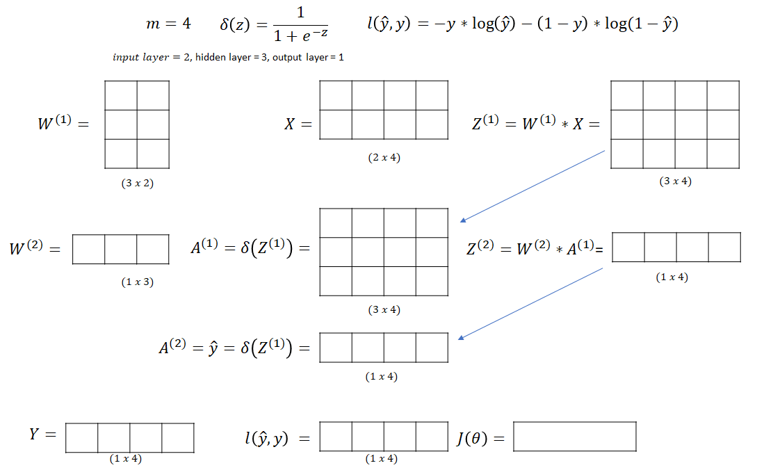
To calculate the output we need to go from the input to the output with all calculations. For example, we define all activation as sigmoid functions, and our loss function as binary cross entropy (the loss function if we have binary output).

For example you have a function to predict that is:

1547485837571

This is a simple function with the binary output (like when you predict if on the image is dog or cat)

def fun_to_predict(x):
  return 1.0 if 3*x[0]*x[1]-2*x[0]>0 else 0.0 #must be float

To calculate the output you need to go through your defined neural network and calculate all the layers.

calculate the first layer by multiply the input with the first layer weights.

1547586657031

Caclulate activation function on the weights.

1547586732170

Calulate the second layer by multiplying the output on the first layer with weights on the second layer.

1547586904341

Calculate the output by activation function in the previous output.

1547586933870

Calculate the cost and lost function.

1547587606618

1547587697072

What’s the difference between cost and loss function?

Usually, they are used interchangeably. But in this case, I thought a cost function as an error on the whole data set as a scalar, but loss function as a single function on one example.

more stackoverflow

Below you can find the example of calculating the output of the 2 layers neural network defined before. You can change values and play with weights on the network.

    def sigmoid(self, s):
        return 1 / (1 + torch.exp(-s))        
      
    def loss_function(self,yhat,y):
        return -y * torch.log(yhat) - (1-y)* torch.log(1-yhat);
   
    def loss(self, yhat,y):
        # Binary classification logistic loss 
        return torch.mean(self.loss_function(yhat,y));
    
    def forward(self, X): # m - number of examples
        # (3 X 2) * (2 x m) = (3 x m)  
        self.z1 = torch.matmul(self.W1 , X) 
        # (3 X m) activation function
        self.a1 = self.sigmoid(self.z1) 
        # (1 x 3) * (3 x m) = (1 x m)
        self.z2 = torch.matmul(self.W2, self.a1) 
        # (1 x m) final activation function
        yhat = self.sigmoid(self.z2) 
        return yhat

import torch
import torch.nn as nn
import torch.nn.functional as F

class Neural_Network(nn.Module):
    def __init__(self, inputSize = 2, outputSize = 1, hiddenSize = 3 ):
        super(Neural_Network, self).__init__()
        # parameters
        self.inputSize = inputSize
        self.outputSize = outputSize
        self.hiddenSize = hiddenSize
        
        # weights
        #self.W1 = torch.randn(self.hiddenSize, self.inputSize) # 3 X 2 tensor
        #self.W2 = torch.randn(self.outputSize, self.hiddenSize) # 1 X 3 tensor
        self.W1 = torch.tensor([[0.5,0.5],[0.6,0.7],[0.6,0.7]])
        self.W2 = torch.tensor([[0.1,0.2,0.3]])
        
    def sigmoid(self, s):
        return 1 / (1 + torch.exp(-s))        
      
    def loss_function(self,yhat,y):
        return -y * torch.log(yhat) - (1-y)* torch.log(1-yhat);
   
    def loss(self, yhat,y):
        # Binary classification logistic loss 
        # Special case of cross entropy 
        # (http://wiki.fast.ai/index.php/Log_Loss)
        # nn.BCELoss()
        return torch.mean(self.loss_function(yhat,y));
    
    def forward(self, X): # m - number of examples
        self.z1 = torch.matmul(self.W1 , X) # (3 X 2) * (2 x m) = (3 x m)  ".dot" does not broadcast in PyTorch
        print('Z1',self.z1)
        
        self.a1 = self.sigmoid(self.z1) # (3 X m) activation function
        print('A1',self.a1)
        
        self.z2 = torch.matmul(self.W2, self.a1) # (1 x 3) * (3 x m) = (1 x m)
        print('Z2', self.z2)
        
        yhat = self.sigmoid(self.z2) # (1 x m) final activation function
        print('A2',yhat)
        
        return yhat    
    
def fun_to_predict(x):
  return 1.0 if 3*x[0]*x[1]-2*x[0]>0 else 0.0 #must be float

NN = Neural_Network(2,1)
X = torch.tensor( [[0.1,0.2,.3,.4],[.5,.6,.7,.8]])
Y = torch.t( torch.tensor( [[fun_to_predict(x)] for x in torch.t(X)]   ) ) # (1 x m)

print('X:',X)
print('Y:',Y)

Yhat = NN.forward(X) #or NN(X)

print('L:',NN.loss_function(Yhat,Y))
print('J:',NN.loss(Yhat,Y))

Gradient Descent more

When you know how to calculate your result is time to update weights to get the best result in your neural network. For this you need to use Gradient Descent. This algorithm is use the fact that if you want find the minimimum of the cost function you can use derivative of the cost function to recognize the direction how to update weights and the value shows how much to update.

Let’s assume that you have only one weight (w), so the cost function J(θ) you can present in a 2D plot. (on the x axis weight, and on the y axis J(θ)).

1548179188819

1548137149402

1548137409720

Where your whole function to calculate the final cost J(θ) is:

1548137505581

Your gradient will be a derivative cost function on your weight.

1548137519406

1548138648303

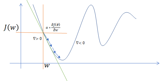
If your gradient is positive, this means that the plot is increasing, so we have to subtract the value of the gradient (go to the left). If your gradient is negative, this means that you need to add the value to your weight (go to the right).

In your final neural network, you have more dimensions, and it is impossible to show it on the single plot.

Backpropagation

When you know how to update weights, it is time to calculate the gradient for your neural network. You need to find the gradient on your weight, but the problem might be your equation that is little more complicated.

Let’s look how you calculate your final cost.

1548183708290

In backpropagation, you need to go back from right to left and on each step calculate derivative to update the previous layer. For this you use the chain rule: wiki

In the chain rule, you can calculate the partial derivative of the composition of two or more functions.

1548140736187

For example in your neural network you if you want to calculate new weights on your first layer and the second layer according to the gradient descent you have to calculate partial derivative on your cost function.

1548193684435

1548193713633

By using chain rule, you can calculate partial derivative based on the partial derivative on each function.

1548194181907

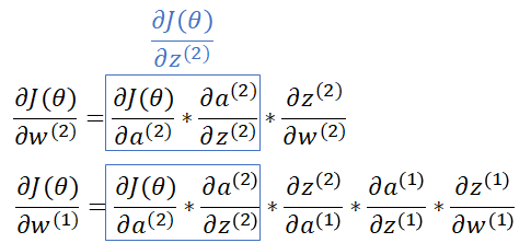
You can go from the right to the left and calculate the error on each step, and next propagate this to the previous layer and update your weights.

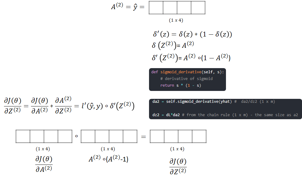
Hadamard product wiki

Sometimes you will see ∘ instead of ∗ in the multiplication between matrices. This sign is a Hadamard product, and by this, you multiply two matrices with the same dimension by multiply each part of matrix themselves. For example if your f(x)=x*(x-1). The matrix calculation wouldn’t be multiple two matrices but Hamarad product of this.

1548182006468

Below you can find an algorithm for a matrix with m examples .

1548182396033

Calculate the error on the cost function

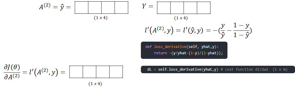
Backpropagate this to calculate the loss on the dJ/Z[2] layer.

Backpropagate to get update for the second Layer W[2]

We go further to update W[1]. First calculate dJ/dA[1]

Next we calculate dJ/dZ[1]

The last step before update is to find the dJ/dW[1]

The final step is to update your weights with new values, and calculate new loss and cost.

import numpy as np
import torch
import torch.nn as nn
import torch.nn.functional as F

class Neural_Network(nn.Module):
    def __init__(self, inputSize = 2, outputSize = 1, hiddenSize = 3 ):
        super(Neural_Network, self).__init__()
        # parameters
        self.inputSize = inputSize
        self.outputSize = outputSize
        self.hiddenSize = hiddenSize
        
        # weights
        #self.W1 = torch.randn(self.hiddenSize, self.inputSize) # 3 X 2 tensor
        #self.W2 = torch.randn(self.outputSize, self.hiddenSize) # 1 X 3 tensor
        self.W1 = torch.tensor([[0.5,0.5],[0.6,0.7],[0.6,0.7]])
        self.W2 = torch.tensor([[0.1,0.2,0.3]])
        
    def sigmoid(self, s):
        return 1 / (1 + torch.exp(-s))        
      
    def loss_function(self,yhat,y):
        return -y * torch.log(yhat) - (1-y)* torch.log(1-yhat);
   
    def loss(self, yhat,y):
        # Binary classification logistic loss 
        # Special case of cross entropy (http://wiki.fast.ai/index.php/Log_Loss)
        # nn.BCELoss()
        return torch.mean(self.loss_function(yhat,y));
    
    def forward(self, X): # m - number of examples
        self.z1 = torch.matmul(self.W1 , X) # (3 X 2) * (2 x m) = (3 x m)  ".dot" does not broadcast in PyTorch
        print('Z1',self.z1)
        
        self.a1 = self.sigmoid(self.z1) # (3 X m) activation function
        print('A1',self.a1)
        
        self.z2 = torch.matmul(self.W2, self.a1) # (1 x 3) * (3 x m) = (1 x m)
        print('Z2', self.z2)
        
        yhat = self.sigmoid(self.z2) # (1 x m) final activation function
        print('A2',yhat)
        
        return yhat   
      
    def sigmoid_derivative(self, s):
        # derivative of sigmoid
        return s * (1 - s)
      
      
    def loss_derivative(self, yhat,y):
        return -(y/yhat-(1-y)/(1-yhat));      
          
      
    def backward(self, X, y, yhat, lr): #lr learning rate
        print('Step 1:')
        # yhat = a2
        dL = self.loss_derivative(yhat,y) # cost function dI/da2  (1 x m)
        print('dL:', dL)

        print('Step 2:')
        da2 = self.sigmoid_derivative(yhat) #  da2/dz2 (1 x m)
        print('dA2:', da2)
        
        dz2 = dL*da2 # dl/dz2 from the chain rule (1 x m) - the same as a2
        print('dz2:', dz2)
        
        print('Step 3:')
        # dL/da2 * da2/dz2 (*) dz2/dW2(T)  [a1]  | (1 x m) * (3 x M)^T = (1 x 3)
        dW2 = torch.matmul(dz2, torch.t(self.a1)) 
        print('dW2:', dW2)
        
        
        print('Step 4:')
        # dl/da1 = dz2/dW2(T) * dL/dz2 | (1x3)^T * (1 x m) = (3 x 1) * (1 x m) = (3 * m)
        da1 = torch.matmul( torch.t(self.W2 ) , dz2 )
        print('da1:', da1)
        
        
        print('Step 5:')
        #  dz1 = dL/da1 * da1/dz1  | (3 x m) * (3 x m) = (3 x m)
        dz1 = da1 * self.sigmoid_derivative(self.a1)
        
        print('sZ1: ', self.sigmoid_derivative(self.a1) );
        print('dZ1: ', dz1 );
        
        print('Step 6:')
        dW1 = torch.matmul(dz1, torch.t(X)  )  # (3 * m) * (m x 2) = (3 x 2)
        print('dW1: ', dW1 );

        
        print('Step 7:')
        self.W1 -= lr*dW1
        print('alpha*dW1: ', lr*dW1 );
        print('W1: ', self.W1 );
        
        self.W2 -= lr*dW2
        print('alpha*dW2: ', lr*dW2 );
        print('W2: ', self.W2 );
        
        return      
    
def fun_to_predict(x):
  return 1.0 if 3*x[0]*x[1]-2*x[0]>0 else 0.0 #must be float

NN = Neural_Network(2,1)
X = torch.tensor( [[0.1,0.2,.3,.4],[.5,.6,.7,.8]])
Y = torch.t( torch.tensor( [[fun_to_predict(x)] for x in torch.t(X)]   ) ) # (1 x m)

print('X:',X)
print('Y:',Y)

print('Forward:')
Yhat = NN.forward(X) #or NN(X)

print('L:',NN.loss_function(Yhat,Y))
print('J:',NN.loss(Yhat,Y))

print('Backward:')
NN.backward(X,Y,Yhat,0.1)


Yhat = NN.forward(X) #or NN(X)
print('L: ', NN.loss_function(Yhat,Y))
print('J: ', NN.loss(Yhat,Y))

Pytorch Implementation

NN = Neural_Network(2,1)
X = torch.randn(2,10) # random values from [0,1] (2 x m)

def fun_to_predict(x):
  return 1.0 if x[0]*x[1]+2*x[0]>0 else 0.0 #must be float

Y = torch.t( torch.tensor( [[fun_to_predict(x)] for x in torch.t(X)]   ) ) # (1 x m)
yhat = NN(X)

print (" Loss: " + str(NN.loss(yhat,Y).detach().item())) 

for i in range(100):  # trains the NN 100 times
  NN.train(X, Y, 1.0)

yhat = NN(X)
print ("#" + str(i) + " Loss: " + str(NN.loss(yhat,Y).detach().item()))

ypred = NN.predict(X)
     
print ("Predicted data based on trained weights: ")
print ("Input: \n" + str(X))
print ("Output: \n" + str(ypred))   
print ("Real: \n" + str(Y))

import torch
import torch.nn as nn
import torch.nn.functional as F

class Neural_Network(nn.Module):
    def __init__(self, inputSize = 2, outputSize = 1, hiddenSize = 3 ):
        super(Neural_Network, self).__init__()
        # parameters
        self.inputSize = inputSize
        self.outputSize = outputSize
        self.hiddenSize = hiddenSize
        
        # weights
        self.W1 = torch.randn(self.hiddenSize, self.inputSize) # 3 X 2 tensor
        self.W2 = torch.randn(self.outputSize, self.hiddenSize) # 1 X 3 tensor
        
    def forward(self, X): # m - number of examples
        self.z1 = torch.matmul(self.W1 , X) # (3 X 2) * (2 x m) = (3 x m)  ".dot" does not broadcast in PyTorch
        self.a1 = self.sigmoid(self.z1) # (3 X m) activation function
        self.z2 = torch.matmul(self.W2, self.a1) # (1 x 3) * (3 x m) = (1 x m)
        yhat = self.sigmoid(self.z2) # (1 x m) final activation function
        return yhat
        
    def sigmoid(self, s):
        return 1 / (1 + torch.exp(-s))
    
    def sigmoid_derivative(self, s):
        # derivative of sigmoid
        return s * (1 - s)
      
    def loss(self, yhat,y):
        # Binary classification logistic loss 
        # Special case of cross entropy (http://wiki.fast.ai/index.php/Log_Loss)
        # nn.BCELoss()
        return torch.mean(-y * torch.log(yhat) - (1-y)* torch.log(1-yhat));

      
    def loss_derivative(self, yhat,y):
        return -(y/yhat-(1-y)/(1-yhat));      
    
    def backward(self, X, y, yhat, lr): #lr learning rate
        # yhat = a2
        dL = self.loss_derivative(yhat,y) # cost function dI/da2  (1 x m)
        
        da2 = self.sigmoid_derivative(yhat) #  da2/dz2 (1 x m)
        dz2 = dL*da2 # dl/dz2 from the chain rule (1 x m) - the same as a2
        
        # dL/da2 * da2/dz2 (*) dz2/dW2(T)  [a1]  | (1 x m) * (3 x M)^T = (1 x 3)
        dW2 = torch.matmul(dz2, torch.t(self.a1)) 
        

        # dl/da1 = dz2/dW2(T) * dL/dz2 | (1x3)^T * (1 x m) = (3 x 1) * (1 x m) = (3 * m)
        da1 = torch.matmul( torch.t(self.W2 ) , dz2 )
        #  dz1 = dL/da1 * da1/dz1  | (3 x m) * (3 x m) = (3 x m)
        dz1 = da1 * self.sigmoid_derivative(self.a1)  
        dW1 = torch.matmul(dz1, torch.t(X)  )  # (3 * m) * (m x 2) = (3 x 2)

        self.W2 -= lr*dW2
        self.W1 -= lr*dW1
        return
     

    def train(self, X, y, lr = 0.1):
        # forward + backward pass for training
        yhat = self.forward(X)
        self.backward(X, y, yhat, lr)
        
    def saveWeights(self, model):
        # we will use the PyTorch internal storage functions
        torch.save(model, "NN")
        # you can reload model with all the weights and so forth with:
        # torch.load("NN")
        
    def predict(self,xPredicted):
        yhat = self.forward(xPredicted)
        y = [1 if y >= 0.5 else 0 for y in torch.t(yhat)]
        return y
              

# torch.manual_seed(123) # set the constant seed for the random (JUST FOR TESTING)

NN = Neural_Network(2,1)
X = torch.randn(2,10) # random values from [0,1] (2 x m)

def fun_to_predict(x):
  return 1.0 if x[0]*x[1]+2*x[0]>0 else 0.0 #must be float

Y = torch.t( torch.tensor( [[fun_to_predict(x)] for x in torch.t(X)]   ) ) # (1 x m)
yhat = NN(X)

print (" Loss: " + str(NN.loss(yhat,Y).detach().item()))  

for i in range(100):  # trains the NN 1,000 times
  NN.train(X, Y, 1.0)

yhat = NN(X)
print ("#" + str(i) + " Loss: " + str(NN.loss(yhat,Y).detach().item()))  

ypred = NN.predict(X)
     
print ("Predicted data based on trained weights: ")
print ("Input: \n" + str(X))
print ("Output: \n" + str(ypred))   
print ("Real: \n" + str(Y))

Loss: 0.7505306005477905
#99 Loss: 0.00372719275765121
Predicted data based on trained weights: 
Input (scaled): 
tensor([[ 1.5810,  1.3010,  1.2753, -0.2010,  0.9624,  0.2492, -0.4845, -2.0929,
         -0.8199, -0.4210],
        [-0.9620,  1.2825, -0.3430, -0.6821, -0.9887, -1.7018, -0.7498, -1.1285,
          0.4135,  0.2892]])
Output: 
[1, 1, 1, 0, 1, 1, 0, 0, 0, 0]
Real: 
tensor([[1., 1., 1., 0., 1., 1., 0., 0., 0., 0.]])

Do I have to implement all these functions?

Fortunately no. All gradient and backpropagation the only think what you have to set up in the Neural Network is:

architecture of the network - How many hidden layer?, What are the activation functions on each layer?
Loss Function - How to calculate loss function in the Neural Network

Optimilization Function - How to update weights. If you choose wrong you can finish in the local minimum instead of the better result
Learning Rate - Find learning rate to use in the neural network

Let’s bring again the same neural network that we define in previous chapter. For all activation we want to use sigmoid function and for loss

1547391156214

1548182396033

Name	Comment
`torch.nn.Linear`	Simple Linear Layer in the neural network more
`torch.nn.Sigmoid`	Sigmoid activation function more
`torch.nn.BCELoss`	Binary classification logistic loss more
`torch.optim.SGD`	stochastic gradient descent more

What’s the difference between stochastic gradient descent adn gradient descent?

Stochastic gradient descent (often shortened to SGD) means that you update set parameters in an iterative for each sample one by one. In Gradient Descent you get your whole data to calculate the loss and update your weights. Quora Question wiki

Using Sequential

inputSize = 2
outputSize = 1
hiddenSize = 3

model = torch.nn.Sequential(
          torch.nn.Linear(inputSize, hiddenSize),
          torch.nn.Sigmoid(),
          torch.nn.Linear(hiddenSize, outputSize),
    	  torch.nn.Sigmoid(),
        )

# define loss function, sinble Binary 
loss_fn = torch.nn.BCELoss()

# Implements stochastic gradient descent (optionally with momentum).
optimizer = torch.optim.SGD(model.parameters(),lr=1e-1)

Using nn.Model

class TwoLayerNet(nn.Module):
  def __init__(self,inputSize = 2, outputSize = 1, hiddenSize = 3):
    super(TwoLayerNet, self).__init__();
    
    # define first layer and second layer
    self.linear1 = torch.nn.Linear(inputSize, hiddenSize)
    self.linear2 = torch.nn.Linear(hiddenSize, outputSize)

  # calculate the output  
  def forward(self, X):
    h = torch.sigmoid(self.linear1(X))
    return torch.sigmoid(self.linear2(h));

#define model
model = TwoLayerNet()

# define loss function, sinble Binary 
loss_fn = torch.nn.BCELoss()

# Implements stochastic gradient descent (optionally with momentum).
optimizer = torch.optim.SGD(model.parameters(),lr=1e-1)

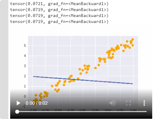
Example of SGD for linear function

example of updating weights for linear function from the fast.ai course.

%matplotlib inline
from fastai.basics import *

n = 100
x = torch.ones(n,2) 
x[:,0].uniform_(-1.,1) # (m x 2) (2 is a number of input parameters)

a = tensor(3.,2); # The parameters that we should find
y = x@a + torch.rand(n) # (m x 1)

def mse(y_hat, y): return ((y_hat-y)**2).mean() # mean square error
a = nn.Parameter(tensor(-1.,1)); # unknown parameter for function y=x@a, (n x 1) = (n x 2) x (2 x 1)

def update(i):
    y_hat = x@a # uour testing, forward function
    loss = mse(y, y_hat) #loss
    if i % 10 == 0: print(loss)
    loss.backward()  # backward functions
    with torch.no_grad(): # with gradient we g
        a.sub_(lr * a.grad) # a.grad - gives information about gration, it will update a, i need to go oposite.
        a.grad.zero_() # zero gradient

lr = 1e-1
        
# ANIMATE
from matplotlib import animation, rc
rc('animation', html='html5')

fig = plt.figure()
plt.scatter(x[:,0], y, c='orange')
line, = plt.plot(x[:,0], x@a)
plt.close()

def animate(i):
    update(i)
    line.set_ydata(x@a)
    return line,

animation.FuncAnimation(fig, animate, np.arange(0, 100), interval=20)

1550262060215

Data / Source

In this chapter I want to brink some information how to get any data to learn, and how to convert them to be helpfull in the learning process.

Resources

List of free resources for your own use.

How to get data and other sources of data for Data-Science and Machine Learning

Name	Description
Medical Data link	List of a lot of medical data that can be used for Machine Learning
Kaggle Datasets link	List a lot of datasets for Kaggle competitions.
Archive DataSet from Wisconsinlink	Archive Data-Set that help you to get data from Wisconsin Library.
fast.ai Datasets more	List of datatsets for image classification/NLP processing
BelgiumTS DataSet link	BelgiumTS DataSet with road signs classification.
Flower Datasets more	flower datasets
Human 3.6MLmore	3.6 million 3D human poses and corresponding images.

Text Resources:

Name	Description
Sentiment Analysis in Text more	`.csv` file with 40,000 text and defined emetions. (`sadness`, `enthusiasm`, `worry`, `love`)
EmoBank more	Large DataBase text with a score for each emotion (`Valence`-`Arousal`-`Dominance`scheme)
EmoInt more	Shared Task on Emotion Intensity, 4 emotions (`anger`, `fear`, `joy`, `sadness`). visualisation

Tabular Data

Name	Description
Movielens more	Non-commercial, personalized movie recommendations.

Data Download / Google Drive

If you use Google Colab you can easly mount your Gdrive in the filesystem. I also create a link for “My Drive”(ln), because it is easier to go to a folder without a space in the name.

# Load the Drive helper and mount
from google.colab import drive
drive.mount('/content/drive')
!ln -s "/content/drive/My Drive/" /content/gdrive

1550258836263

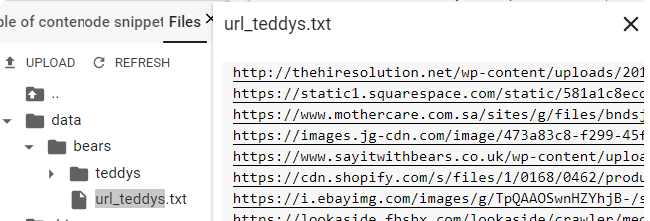
Data Download / Google Images

You can also download using google images search engine. For this,

Prepare folder structure for your classes.

from fastai.vision import *

folder = 'teddys'

path = Path('data/bears')
dest = path/folder
dest.mkdir(parents=True, exist_ok=True)

1550259522813

Go to google images, find interesting search images, go to the developer consolectrl+shift+j and type:

urls = Array.from(document.querySelectorAll('.rg_di .rg_meta')).map(el=>JSON.parse(el.textContent).ou);
window.open('data:text/csv;charset=utf-8,' + escape(urls.join('\n')));

1550259689567

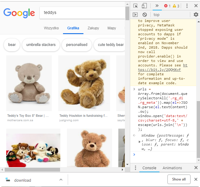
This wll download you the file download, rename the file to urls_teddys.txt and upload to your path in the jupyter or colab

1550259797554

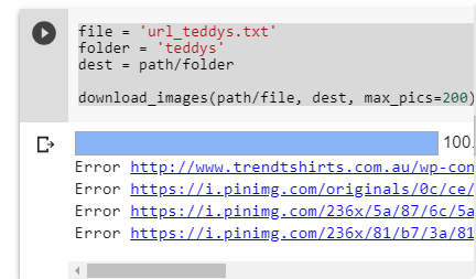
Download your files using download_images

file = 'url_teddys.txt'
folder = 'teddys'
dest = path/folder

download_images(path/file, dest, max_pics=200)

1550259892436

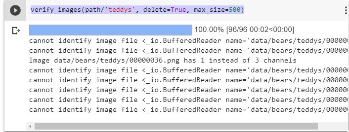
The last step is to verify images. This will remove images that are corrupted or doesn’t have 3 channels.

verify_images(path/'teddys', delete=True, max_size=500)

1550260036514

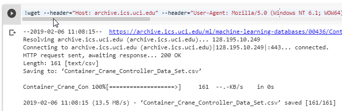
Data Download / wget

There is an extension for the chrome that you can get to generate wget command for your Linux command line. Just add the extension and after start downloading cancel this and copy the command to your console. (or in the Jupyter Notebook with exclamation character “!”).

1549318371426

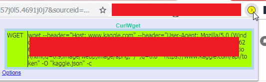
!wget --header="Host: archive.ics.uci.edu" --header="User-Agent: Mozilla/5.0 (Windows NT 6.1; WOW64) AppleWebKit/537.36 (KHTML, like Gecko) Chrome/72.0.3626.81 Safari/537.36" --header="Accept: text/html,application/xhtml+xml,application/xml;q=0.9,image/webp,image/apng,*/*;q=0.8" "https://archive.ics.uci.edu/ml/machine-learning-databases/00436/Container_Crane_Controller_Data_Set.csv" -O "Container_Crane_Controller_Data_Set.csv" -c

1549482301055

Data Download / kaggle

!pip install kaggle

Sign to the profile on the Kaggle page:

1549317920891

Next, download new API key. Upload

1549317857572

And upload to your page: (On Colab you can upload your page)

1549317981152

Copy the kaggle configuration to the home folder.

!mkdir ~/.kaggle
!cp /content/kaggle.json ~/.kaggle/kaggle.json
!chmod 600 ~/.kaggle/kaggle.json

Now you can download any competion that you are in: (kaggle will create folders by themself)

!kaggle competitions download -c home-credit-default-risk -p /content/titanic

Errors:

Error 401 - means that you have wrong .json file. Generate again and check if exists.
Error 403 - You don’t accept terms and condition for the competition. Go to the webpage and join to the competition.

Data Download / linux commands

Useful commands to operate on files.

Command	Example	Description
`Create Directory`	`mkdir folder`	Create directory named `folder`
`Remove files`	`rm content/*.zip`	Remove all files with extension ``.zip`
`Unizip files`	`unzip -o -q isic-images.zip -d isd/bening`	Unzip the files `isic-images.zip`, the `-o` option is used to suppress the query, the `-q` is used to not show list of extracted files, `-d` is a destination folder
`Move files`	`mv isd/benign/ISIC-images/*/.jpg isd/benign`	Move all files with the extension `.jpg` from the folder `isd/benign/ISIC-images` , the double start `**` means to tro find files in the folder and subfolder recseively., Destination folder is `isd/benign`
`Copy files`	`cp isd/benign/ISIC-images/*/.jpg isd/benign`	The same as above without remove original files.

Architecture

Glossary

Name	Description
`parameters`	Configuration of the Neural network (Contains `weights` and `biases`)
`activation function`	Function to activate
`activation`	Result of the `activation functions`
`input layer`	Input for the Nueral network (called `layer 0`, `x`)
`output layer`	Output of the Neural network (`y`). Activation of the last layer.
`loss function`	Function thant compares `output` with `ground truth`
`embedding` more	Type of the layer that output is a product of two matrices. `X@W`, (e.g.`(5x1)@(5x8)=(8x1)`)

1551271030999

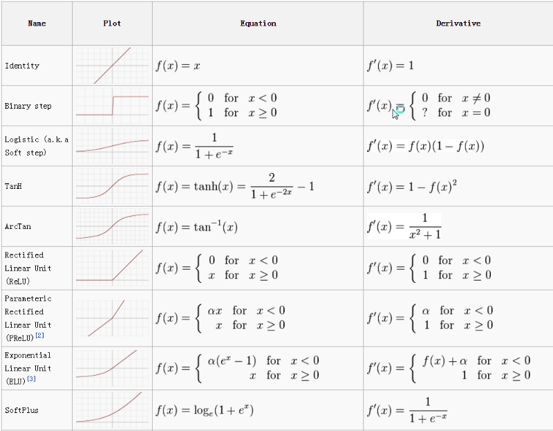
Activation Functions more

Instead of using perceptron with output 0 or 1, better is use activation function that return values between 0 and 1. In Deep learning there are couple functions to use as an activation.

Sigmoid function

In sigmoid function the difference is in the activation function.

Logistic function is:

$f(./assets/6f42e36c949c94189976ae00853af9a1b618e099.svg)={\frac {L}{1+e^{-k(x-x_{0})}}}$

Sigmoid is a special case when L=1, k=1, and x0 = 0.

1543948420834

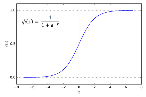
σ = 0.652

When Use?

predict the probability of the output. (simple classification for example: ‘dog/cat’).

List of Activation functions source

When Use?

Currently in the architecture except the last layer, ReLU is the most popular.
For last layer (output) ReLU is not used because we want to have output in the range (e.g. [0,1]), most popular is Sigmoid (Logistic).
Identiny is linear, it can be used for linear regression.

Loss functions more PyTorch

Name	Pytorch	Where Use?
Mean Absolute Error	`nn.L1Loss`	Regression Problems (very rare)
Mean Square Error Loss	`nn.MSELoss`	Regression Problems
Smooth L1 Loss	`nn.SmoothL1Loss`	Regression Problems
Negative Log-Likelihood Loss	`nn.NLLLoss`	Classification
Cross-Entropy Loss	`nn.CrossEntropyLoss`	Classification
Kullback-Leibler divergence	`nn.KLDivLoss`	Classification
Margin Ranking Loss	`nn.MarginRankingLoss`	GANs, Ranking tasks
Hinge Embedding Loss	`nn.HingeEmbeddingLoss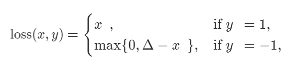`	Learning nonlinear embeddings
Cosine Embedding Loss	`nn.CosineEmbeddingLoss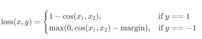`	Learning nonlinear embeddings

weight decay - SGD - L2 Regularization

SGD is a simple loss.backward() that goes backpropage through the model and update weights. If we define a loss as mean squared error:

1551806539435

Weight decay is a regularization term that penalizes big weights. When the weight decay coefficient is big, the penalty for big weights is also big, when it is small weights can freely grow.

There is no difference between L2 regularization and weight decay, in L1 regularization there is absolute value |w| instead of w^2.

1551806603749

Momentum more

Momentum is intended to help speed the optimisation process through cases, to avoid getting stuck in the "shallow valleys" when gradient is close to 0. Momentum accumulates the gradient of the past steps to determine the direction to go.

You update your weights based on the 90% of your previous result (default) and in 10% of your current gradient descent result. In the first time when you don’t have previous result you update in 100% by your gradient descent.

1551965981091

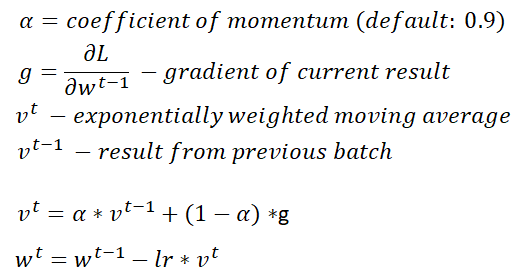
opt = optim.SGD(model.parameters(), lr, momentum=0.9)

RMSProp

Here instead of multiply by momentum we multiply by gradient divident by the root square of the previous result of the batch. In this case we multiply by the square of gradient. This mean that if you are going in the right direction make the number bigger.

If the gradient is really small and St is a small number than the update will be small
If the gradient the gradient is constenely very small and not volatile let’s get bigger jumps.

1551975097200

optimizer = optim.RMSprop(model.parameters(), 
                          lr = 0.0001, 
                          alpha=0.99, 
                          eps=1e-08, 
                          weight_decay=0, 
                          momentum=0)

Adam Optimizer

Adam this combination of RMSProp and Momentum, it’s in less epochs than both separetely.

1551967342004

The final calculation you can find with epsilon value (default 1e-10):

betas coefficients used for computing running averages of gradient and its square (default: (0.9, 0.999)), in the above calculation bheta1, and bheta2.

1551966978062

optimizer = optim.Adam(model.parameters(), lr = 0.0001, betas=(0.9, 0.999), eps=1e-08, weight_decay=0)

Convolution Network more

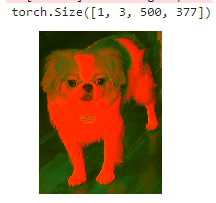
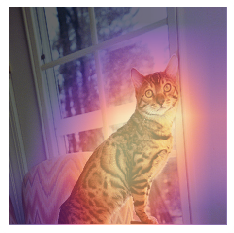
Convolution Network is type of layer in the neural network that can help you to read information about image by putting a mask (like in the most popular image software ) called kernel https://en.wikipedia.org/wiki/Kernel_(image_processing) . It doesn’t have to bet a 3x3 matrix, but this is most popular. In the webpage http://setosa.io/ev/image-kernels/ you can play with the own matrix. The calculation is don for each pixel in the image. For each of them we get the matrix around the pixel with the size of the kernel (3x3) and multiply each of them. The sum is the new pixel of the image.

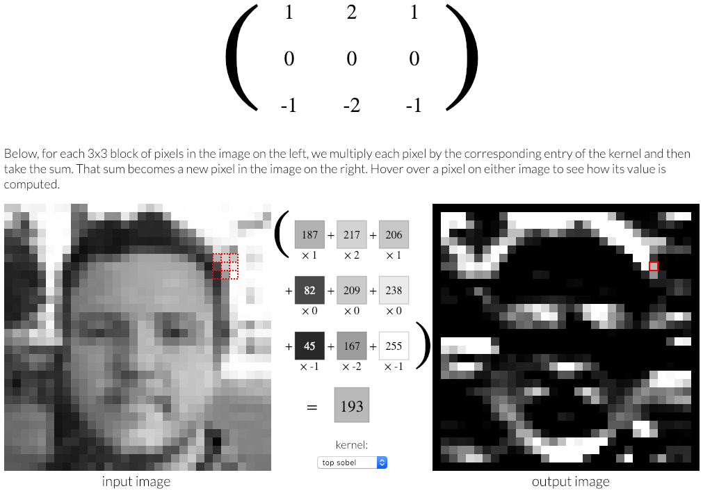
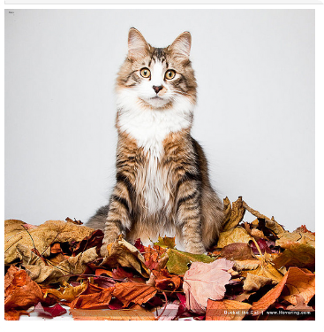
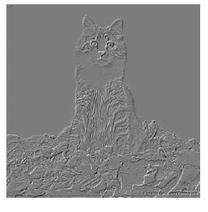
For example below matrix creates from your image of cat edges around your cat.

1552500642360

1552500673214

1552500687431

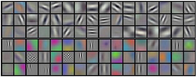
Define different matrix you can find different factors that appear on your image. In the popular models first layer can detect simple artifacts like edges more, but next layers can go into some deeper knowledge like if this is a cat or dog, based on this artifacts. In below example there are 96 kernels with image 11x11x3 that shows different aspects.

F.conv2d

In pytorch function for calculation convolution is F.conv2d,

parameter	definition
`input`	input data
`weight`	kernel to use on the shape
`bias`	optional bial
`stride`	The stride of the convolving kerenl.
`padding`	implicit zero padding on both sides of the input.
`dilation`	the space between kernel elements
`groups`	split input into groups

k = tensor([
    [0.  ,-5/3,1],
    [-5/3,-5/3,1],
    [1.  ,1   ,1],
]).expand(1,3,3,3)/6
F.conv2d(t[None], k,stride=(1,1),padding=1)

1552559867051

stride

Usual your kernel is shifted by 1 pixel (stride=1). Your kernel is start from the position (0,0) and move to the position (1,0) but you can shift the pixel by any value you want.

1552564165730

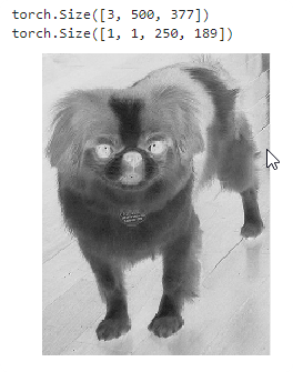
If you set a stride to 2 your kernell will be moved by 2 pixels, and the size of the input image will be 2 times smaller (for example for above image is [250,189]).

1552564234896

output = F.conv2d(t[None],k, 
                  stride=(2,2),
                  padding=1) #shape: ([1, 1, 500, 377])

padding

The default padding for function is 0. The problem is that your image will decrease in the size by 1 pixel for each corner (if you have kernel=(3,3))

[from (10,10) to (9,9)]

1552565495070

To avoid this we can add padding, increase the previous size with 0 values.

1552565871005

The output size is the same as the input size. For 5x5 kernel, the padding must be (2,2) to get the same size of the image.

1552566061084

nn.Conv2d

To create a layer for your model you have a function nn.Conv2d,

n = nn.Conv2d(in_channels = 3,
              out_channels=3,
              kernel_size = (3,3),
              padding=1, stride = 1)

show_image(n(t[None])[0])

1552560544169

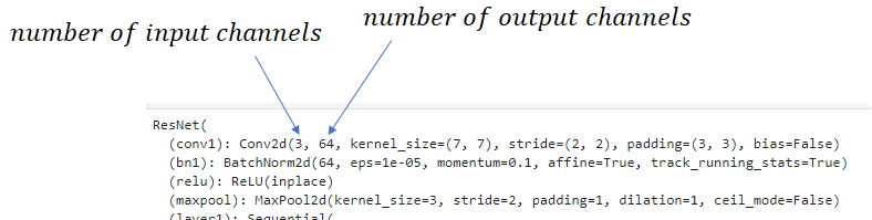
show_image can only accept 1 channel and 3 channels, but you can create more and if you look into resnet34 you will find that first convolution layer has 64 channels as output, and 3 as an input.

from fastai.vision import *

model = models.resnet34()
print(model)

1552567407873

The size of the output more

When you look into summary for your model summary() in the fast.ai you will find the layers that represents convolutional network 2d and size of each layer.

learn.summary()

1552647460580

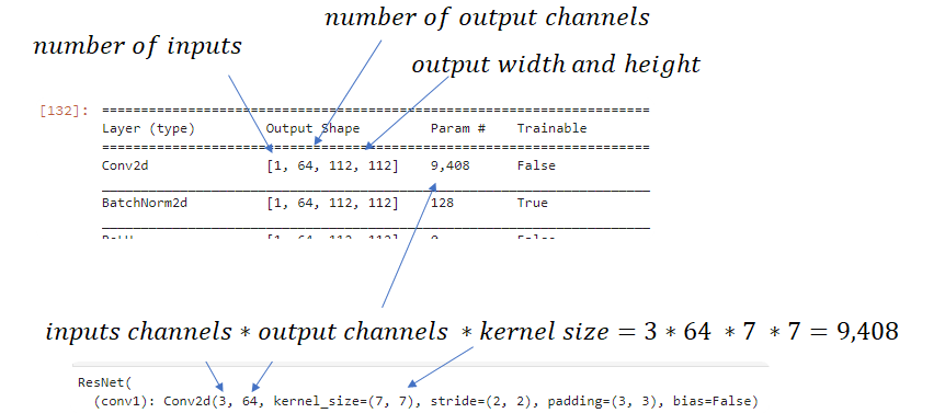
To calculate the output size of the image (width and height), you can use below formula.

1552571969347

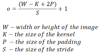
Calculation of Param# for layers: more

Conv: kernel_size*kernel_size*ch_in*ch_out
Linear: (n_in+bias) * n_out
Batchnorm: 2 * n_out
Embeddings: n_embed * emb_sz

Examples:

t = torch.ones(1,3,100,100) #items, channels, width, height
layer = nn.Conv2d(
          in_channels =3,
          out_channels=3,
          kernel_size = (3,3),
          padding=(1,1), 
    	  stride = (1,1))

layer(t).shape

W = 100, H = 100, K=(3,3), P=(1,1), S=(1,1)

ow = (W-K+2P)/S + 1 = (100-3+2)/1+1=100 oh = (W-K+2P)/S + 1 = (100-3+2)/1+1=100

(items, channels,width,height): [1,3,100,100]
out_channels: 64

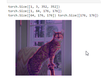
kernel	stride	padding	Output size	calc
`[3,3]`	`(1,1)`	`(1,1)`	`[1, 64, 100, 100]`	`((100-3+2*1)/1+1)`
`[7,7]`	`(1,1)`	`(1,1)`	`[1,64,96,96]`	`((100-7+2*1)/1+1)`
`[3,3]`	`(2,2)`	`(1,1)`	`[1,64,50,50]`	`((100-3+2*1)/2+1)`
`[3,3]`	`(1,1)`	`(0,0)`	`[1,64,49,49]`	`((100-3+2*0)/1+1)`

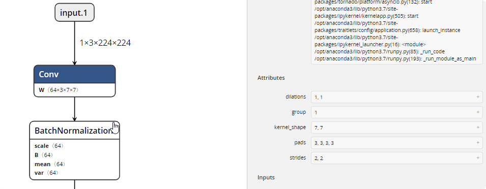
NETRON

You can also show your model in the NETRON APPLICATION https://github.com/lutzroeder/netron as a graph. For the pytorch learn.save() the application show error for me, but you can export your model to the ONNX format, and open in the application.

dummy_input = torch.randn(1, 3, 224, 224).cpu() # the size of your input

torch.onnx.export(learn.model.cpu(), 
                  dummy_input, 
                  "./models/resnet34-entire-model.onnx", 
                  verbose=True)

1552575612810

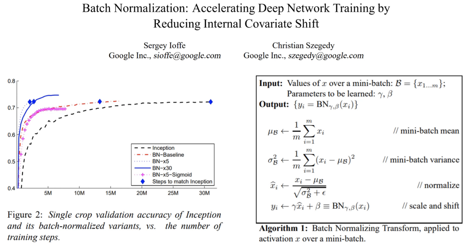
Batch Normalization more paper video

Batch normalization is a type of layer for the neural network that make loss surface smootherby normalizing parameters inside hidden layers, like you do with the input layer.

1552580302141

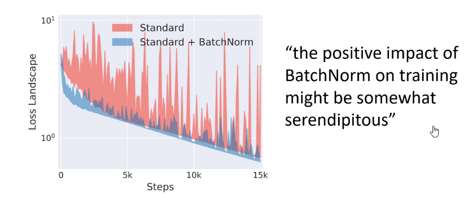
Bath Normalization reduce problem when input changes, so the loss function is more stable and less bumpy.

Batch normalization doesn’t reducing internal covariate shift

Internal Covariate shift refers to change in the distribution of layer inputs caused by updates to the preceding layers. (where for example you put different style of images next time)

Last papers shows that Batch Normalization doesn’t reduce ICS like in the original paper. https://arxiv.org/pdf/1805.11604.pdf](https://arxiv.org/pdf/1805.11604.pdf)

Benefits:

We can use higher learning rates because batch normalization makes sure that there’s no activation that’s gone really high or really low. And by that, things that previously couldn’t get to train, it will start to train.
It reduces overfitting because it has a slight regularization effects.

How it is calculated:

We get mini-batch
Calculate mean (e) anv variance (var) of the mini-batch
normalize the output y=(x-e)/sqrt(var)
Scale and shift the output using own parameters γ and β . This are wieghts that are also larned during a backward optimalization. We also need to scale and shift the normalized values otherwise just normalizing a layer would limit the layer in terms of what it can represent.

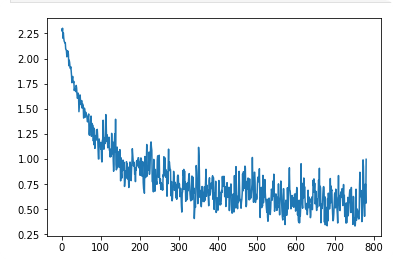
Dropout paper video

1552583126804

Dropout is a tregulariation method that for reducing overfitting in neural network, by preventing complex co-adaptaions on training data. At random, we throw away some percentage of the activations, After we finish traiing we remove dropout on the activation, because we wanted to be accurate. Dropout use Bernoulli distribution to remove some activations.

It helps working with overfitting. If we over fit some parts are recognizing particular image. If we turn off them during training the network the network will avoid this behaviour.

torch.manual_seed(7)
m = nn.Dropout(p=.5) # in 50% probability return 0.
input = torch.randn(4, 2)
m(input)

1552588690527

PyTorch WebPage

Functions

PyTorch is an optimized tensor library for deep learning using GPUs and CPUs.

import torch

Command	Info	Description
`torch.cuda.is_available()`	#	Is CUDA Available (`On CPU returns False`)
`torch.backends.cudnn.enabled`	#	Is CUDA® Deep Neural Network library Available (used by fast.ai, `On CPU returns False`)
`torch.cuda.device_count()`	#	Number of GPUs
`torch.cuda.get_device_name(device)`	#	Gets the name of a device number
`torch.cuda.set_device(device)`	#	Set the current GPU device
`defaults.device = torch.device('cpu')`		Set default device to CPU
`torch.manual_seed(n)`		Set manual seed for random initialization for weights, and oher random calculations.

How to train a model?

In this example there will be creation of model for PyTorch without using fastai library from basics. 1st you need download your data http://deeplearning.net/data/mnist/mnist.pkl.gz. and unpack in your folder.

We can load our data using gzip library, and pickle, mnist.pkl is a pickle file that have been divided into train and validation. We can load them separetely.

import gzip
import pickle
import matplotlib.pyplot as plt

path ='./mnist.pkl.gz'

with gzip.open(path, 'rb') as f:
    ((x_train, y_train), (x_valid, y_valid), _) = pickle.load(f, encoding='latin-1')
    
plt.imshow(x_train[0].reshape((28,28)), cmap="gray")

1551976476263

DataSet / DataLoader

For PyTorch we need to convert the data into Tensor and prepare DataSet, and DataLoader for our model.

DataSet -is used for get original values,
DataLoader - is a class that returns values during training, we don’t want to load the whole dataset into graphics memory, and second we can do some transformation (like data augmentation) before return to the model.

import torch
import torch.nn as nn
from torch.utils import data

# CUDA for PyTorch
use_cuda = torch.cuda.is_available()
device = torch.device("cuda:0" if use_cuda else "cpu")

x_train,y_train,x_valid,y_valid = map(torch.tensor, (x_train,y_train,x_valid,y_valid))


bs=64

# # We can use simple TensorDataset, instead of creating own
class DatasetXY(data.Dataset):
  'Characterizes a dataset for PyTorch'
  def __init__(self, X, Y):
        'Initialization'
        self.X = X
        self.Y = Y

  def __len__(self):
        'Denotes the total number of samples'
        return len(self.X)

  def __getitem__(self, index):
        'Generates one sample of data'
        # Select sample
        x = self.X[index]
        y = self.Y[index]
        return x.to(device), y.to(device)

train_ds = DatasetXY(x_train,y_train)
valid_ds = DatasetXY(x_valid,y_valid)

# we ccan use this isntead of DatasetXY
#train_ds = data.TensorDataset(x_train, y_train)
#valid_ds = data.TensorDataset(x_valid, y_valid)
    
train_dl = data.DataLoader(train_ds,batch_size=bs)
valid_dl = data.DataLoader(valid_ds,batch_size=bs)

Model

Next, we define our model, with one linear layout, cuda() is required to work model in graphics card.

# Our model
class Mnist_Logistic(nn.Module):
    def __init__(self):
        super().__init__()
        self.lin = nn.Linear(784, 10, bias=True)

    def forward(self, xb): return self.lin(xb)

    model = Mnist_Logistic().cuda()

Backward propagation

The last option is to update our weights, learn algorithm, and prepare loss function. nn.CrossEntropyLoss()


lr=2e-2
loss_func = nn.CrossEntropyLoss()

def update(x,y,lr):
    wd = 1e-5
    y_hat = model(x)
    # weight decay
    w2 = 0.
    for p in model.parameters(): w2 += (p**2).sum() #weight decay
    # add to regular loss
    loss = loss_func(y_hat, y) + w2*wd
    #print(loss.item())
    loss.backward()
    with torch.no_grad():
        for p in model.parameters():
            p.sub_(lr * p.grad)
            p.grad.zero_()
    return loss.item()

Now we can learn our model, based on the training data loader.

Learn

def get_batch(dl):
    for x,y in dl: yield x.to(device),y.to(device)

losses = [update(x,y,lr) for x,y in get_batch(train_dl)]
plt.plot(losses);

import gzip
import pickle
import matplotlib.pyplot as plt
# from fastai.basics import *

path ='./mnist.pkl.gz'

with gzip.open(path, 'rb') as f:
    ((x_train, y_train), (x_valid, y_valid), _) = pickle.load(f, encoding='latin-1')
    
plt.imshow(x_train[0].reshape((28,28)), cmap="gray")

import torch
import torch.nn as nn
from torch.utils import data

# CUDA for PyTorch
use_cuda = torch.cuda.is_available()
device = torch.device("cuda:0" if use_cuda else "cpu")

x_train,y_train,x_valid,y_valid = map(torch.tensor, (x_train,y_train,x_valid,y_valid))


bs=64

# # We can use simple TensorDataset, instead of creating own
class DatasetXY(data.Dataset):
  'Characterizes a dataset for PyTorch'
  def __init__(self, X, Y):
        'Initialization'
        self.X = X
        self.Y = Y

  def __len__(self):
        'Denotes the total number of samples'
        return len(self.X)

  def __getitem__(self, index):
        'Generates one sample of data'
        # Select sample
        x = self.X[index]
        y = self.Y[index]
        return x.to(device), y.to(device)

train_ds = DatasetXY(x_train,y_train)
valid_ds = DatasetXY(x_valid,y_valid)

# we ccan use this isntead of DatasetXY
#train_ds = data.TensorDataset(x_train, y_train)
#valid_ds = data.TensorDataset(x_valid, y_valid)
    
train_dl = data.DataLoader(train_ds,batch_size=bs)
valid_dl = data.DataLoader(valid_ds,batch_size=bs)

# Our model
class Mnist_Logistic(nn.Module):
    def __init__(self):
        super().__init__()
        self.lin = nn.Linear(784, 10, bias=True)

    def forward(self, xb): return self.lin(xb)

model = Mnist_Logistic().cuda()


lr=2e-2
loss_func = nn.CrossEntropyLoss()

def update(x,y,lr):
    wd = 1e-5
    y_hat = model(x)
    # weight decay
    w2 = 0.
    for p in model.parameters(): w2 += (p**2).sum() #weight decay
    # add to regular loss
    loss = loss_func(y_hat, y) + w2*wd
    #print(loss.item())
    loss.backward()
    with torch.no_grad():
        for p in model.parameters():
            p.sub_(lr * p.grad)
            p.grad.zero_()
    return loss.item()

def get_batch(dl):
    for x,y in dl: yield x.to(device),y.to(device)

losses = [update(x,y,lr) for x,y in get_batch(train_dl)]
plt.plot(losses);

1551982934877

Using 2 layer model

We can define different model and work on it.

import torch.nn.functional as F


class Mnist_NN(nn.Module):
    def __init__(self):
        super().__init__()
        self.lin1 = nn.Linear(784, 50, bias=True)
        self.lin2 = nn.Linear(50, 10, bias=True)

    def forward(self, xb):
        x = self.lin1(xb)
        x = F.relu(x)
        return self.lin2(x)
    
model = Mnist_NN().cuda()

losses = [update(x,y,lr) for x,y in get_batch(train_dl)]
plt.plot(losses);

1551983216377

Adam optimizer

We can also use Adam optimizer instead of our own function to update.

from torch import optim

def update(x,y,lr):
    opt = optim.Adam(model.parameters(), lr)
    y_hat = model(x)
    loss = loss_func(y_hat, y)
    loss.backward()
    opt.step()
    opt.zero_grad()
    return loss.item()

losses = [update(x,y,1e-3) for x,y in get_batch(train_dl)]
plt.plot(losses);

import gzip
import pickle
import matplotlib.pyplot as plt
# from fastai.basics import *

path ='./mnist.pkl.gz'

with gzip.open(path, 'rb') as f:
    ((x_train, y_train), (x_valid, y_valid), _) = pickle.load(f, encoding='latin-1')
    
#plt.imshow(x_train[0].reshape((28,28)), cmap="gray")

import torch
import torch.nn as nn
from torch.utils import data

# CUDA for PyTorch
use_cuda = torch.cuda.is_available()
device = torch.device("cuda:0" if use_cuda else "cpu")

x_train,y_train,x_valid,y_valid = map(torch.tensor, (x_train,y_train,x_valid,y_valid))


bs=64

# # We can use simple TensorDataset, instead of creating own
class DatasetXY(data.Dataset):
  'Characterizes a dataset for PyTorch'
  def __init__(self, X, Y):
        'Initialization'
        self.X = X
        self.Y = Y

  def __len__(self):
        'Denotes the total number of samples'
        return len(self.X)

  def __getitem__(self, index):
        'Generates one sample of data'
        # Select sample
        x = self.X[index]
        y = self.Y[index]
        return x.to(device), y.to(device)

train_ds = DatasetXY(x_train,y_train)
valid_ds = DatasetXY(x_valid,y_valid)

# we ccan use this isntead of DatasetXY
#train_ds = data.TensorDataset(x_train, y_train)
#valid_ds = data.TensorDataset(x_valid, y_valid)
    
train_dl = data.DataLoader(train_ds,batch_size=bs)
valid_dl = data.DataLoader(valid_ds,batch_size=bs)

# Our model
class Mnist_Logistic(nn.Module):
    def __init__(self):
        super().__init__()
        self.lin = nn.Linear(784, 10, bias=True)

    def forward(self, xb): return self.lin(xb)

model = Mnist_Logistic().cuda()


lr=2e-2
loss_func = nn.CrossEntropyLoss()

from torch import optim

def update(x,y,lr):
    opt = optim.Adam(model.parameters(), lr)
    y_hat = model(x)
    loss = loss_func(y_hat, y)
    loss.backward()
    opt.step()
    opt.zero_grad()
    return loss.item()

def get_batch(dl):
    for x,y in dl: yield x.to(device),y.to(device)

losses = [update(x,y,1e-3) for x,y in get_batch(train_dl)]
plt.plot(losses);

1551983650860

Using model with fastai

We can also use our model with fastai library, instead of creating our.

data = DataBunch.create(train_ds, valid_ds, bs=bs) # We don't need create our own loader

loss_func = nn.CrossEntropyLoss()

class Mnist_NN(nn.Module):
    def __init__(self):
        super().__init__()
        self.lin1 = nn.Linear(784, 50, bias=True)
        self.lin2 = nn.Linear(50, 10, bias=True)

    def forward(self, xb):
        x = self.lin1(xb)
        x = F.relu(x)
        return self.lin2(x)

learn = Learner(data, Mnist_NN(), loss_func=loss_func, metrics=accuracy)
learn.lr_find()
learn.recorder.plot()

learn.fit_one_cycle(1, 1e-2)

1551984419055

1551984427879

fast.ai github

Fast.ai is a very popular library for deep learning based on the PyTorch. The library simplifies training fast and accurate neural nets using modern best practices. fast.ai doesn’t replace any base functionality from the PyTorch. It adds a lot of functions that can help you build a model faster.

Requires Python >=3.6 (python --version)

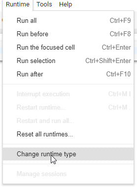
Installation / Google Colab source

On Google Colab you don’t have to install fast.ai. It is installed already. Google Colab gives you Tesla K80 machine with 12GB of GPU RAM.

Go to a page: https://colab.research.google.com
Create new Python 3 notebook

1548781198400

Make sure that you have setup GPU mode

1548781236103

1548781252590

Check version

import fastai
print('fastai: version: ', fastai.__version__)

1548787769768

Test some code from the fast.ai course:


%reload_ext autoreload
%autoreload 2
%matplotlib inline

from fastai import*
from fastai.vision import *

bs = 64
# bs = 16   # uncomment this line if you run out of memory even after clicking Kernel->Restart

path = untar_data(URLs.PETS); path
path_anno = path/'annotations'
path_img = path/'images'


fnames = get_image_files(path_img)
np.random.seed(2)
pat = r'/([^/]+)_\d+.jpg$'


data = ImageDataBunch.from_name_re(path_img, 
                                   fnames, pat, 
                                   ds_tfms=get_transforms(), 
                                   size=224, 
                                   bs=bs
                                  ).normalize(imagenet_stats)

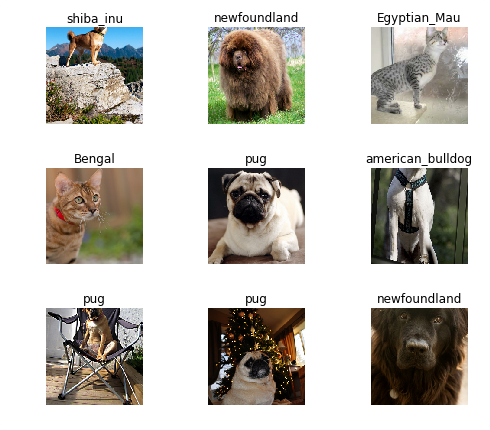
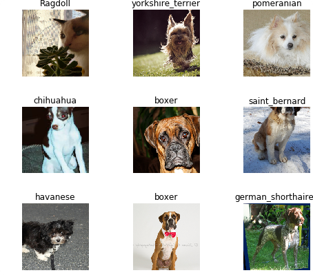
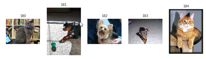
data.show_batch(rows=3, figsize=(7,6))

1548781400369

print(data.classes)
#len(data.classes),data.c

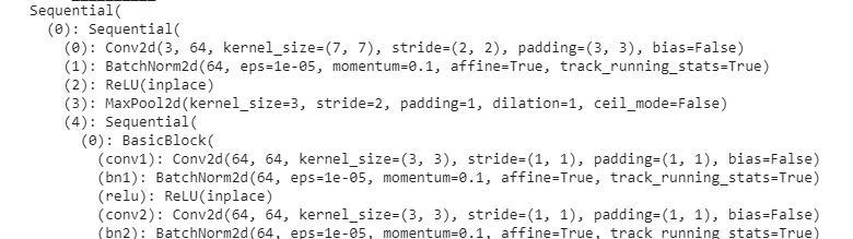
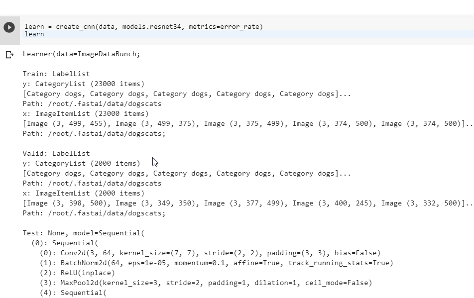
learn = create_cnn(data, models.resnet34, metrics=error_rate)
print(learn.model)

1548781504899

learn.fit_one_cycle(1)
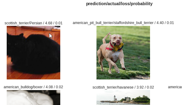
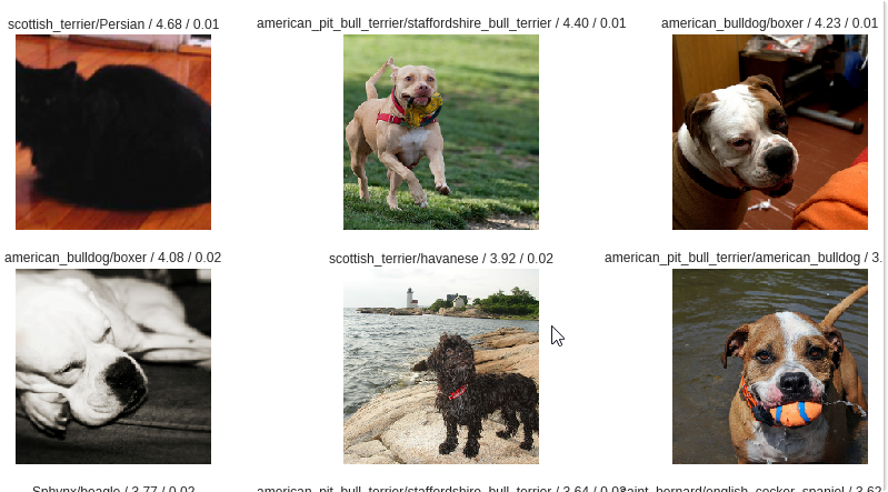
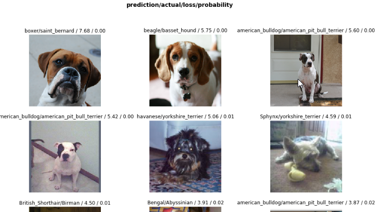
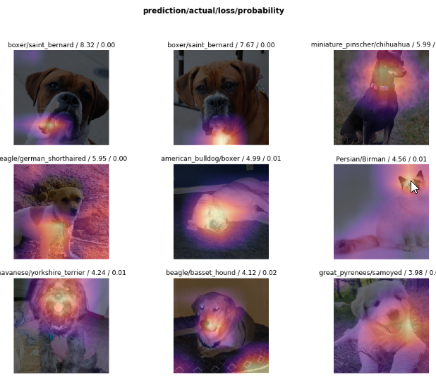
interp = ClassificationInterpretation.from_learner(learn)
losses,idxs = interp.top_losses()


interp.plot_top_losses(9, figsize=(15,11))

1548781518290

1548791676403

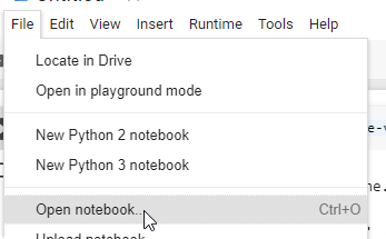
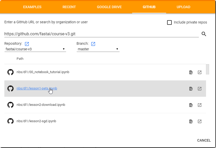
You can open the github repo directly from the course https://github.com/fastai/course-v3.git

1548782192774

1548782244713

Or Upload from your computer

1548782293026

1548788564305

installion / AWS

AWS Free Tier doesn’t include GPU computer

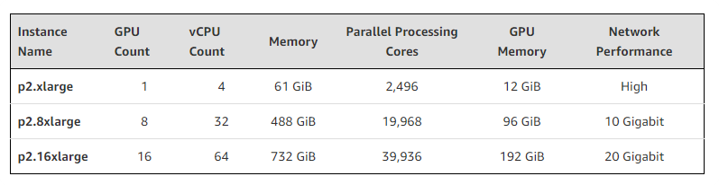
The instance called p2.xlarge that is dedicated for the deep learning cost about 0.9$ per hour. . First you need request to increase the service limit.

p2.xlarge has the NVIDIA GK210 Tesla K80 GPU Machine

1548792962650

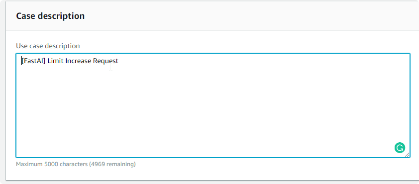
When you login for your AWS as a Free Tier you don’t have acces to create instance called p2.xlarge. First go to the dashboard and request for new limit for this instance.

1548782638507

1548782656757

1548782674826

In your request form choose the best Region, Instance Type, and New Limit Value.

1548782883630

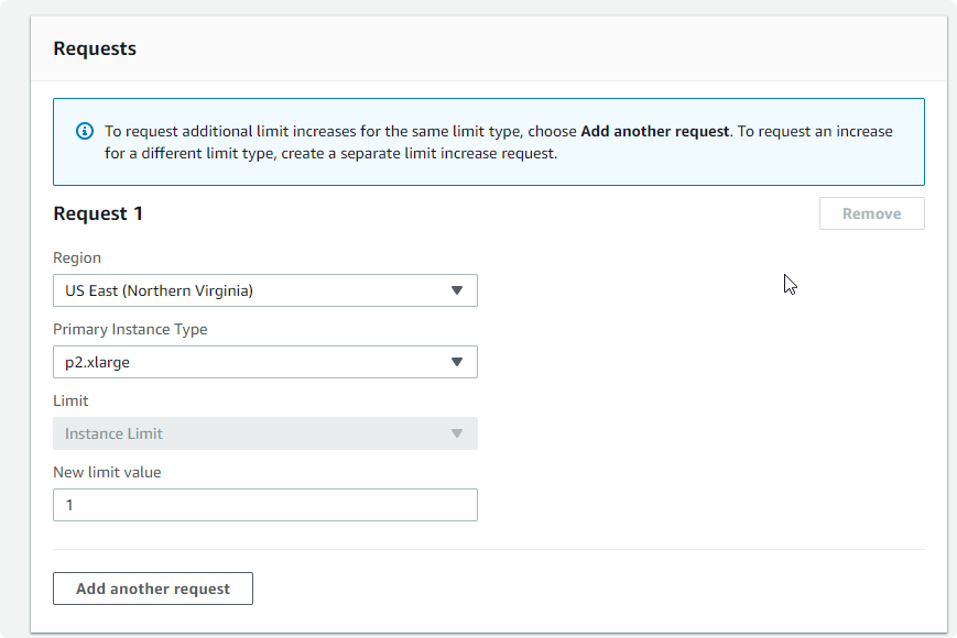
In the description you can type: ‘[FastAI] Limit Increase Request’

1548782954025

After couple of days (usually one) you will get new limit for your Free Tier (This will still charge you for this computer)

After you have ability to create new p2.xlarge instance, you can create new one.

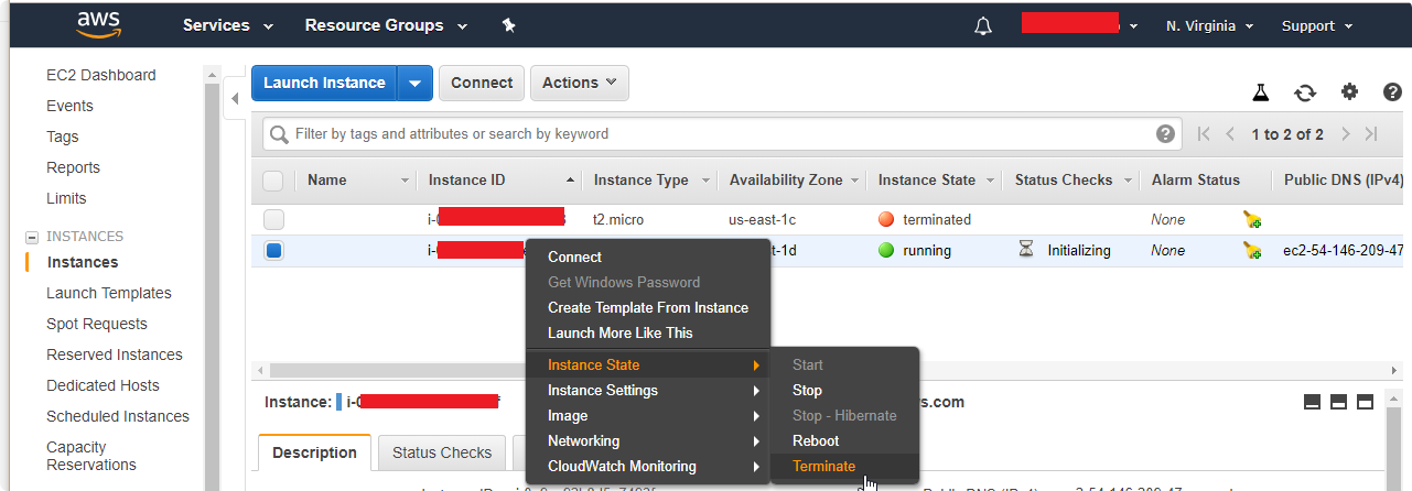
In the services click EC2, and next instances

1548783181553

1548783218231

and click Launch instance

1548783245159

In a list find deep learning instances

1548783307267

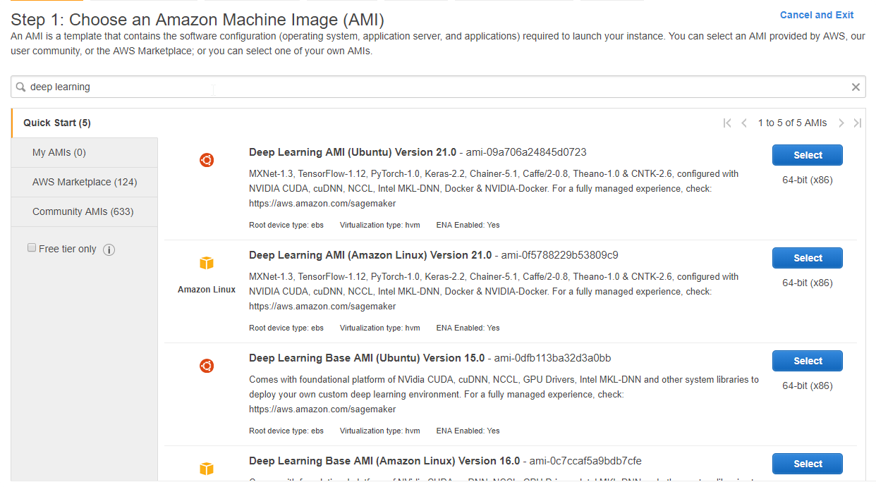
And select newest one:

1548783324760

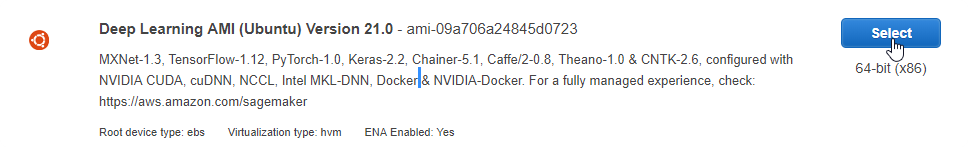
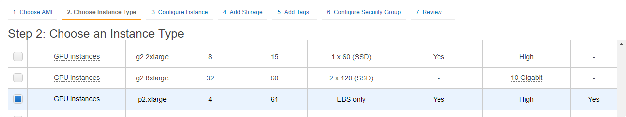
In the Instance type choose p2.xlarge and click Next: Configure Instance details

1548783390814

We don’t change anything in Instance Details, just click next

1548783484833

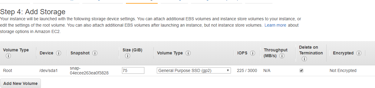
In the storage we stay as it is ( 75 GB).

1548783505382

We don’t add any tags.
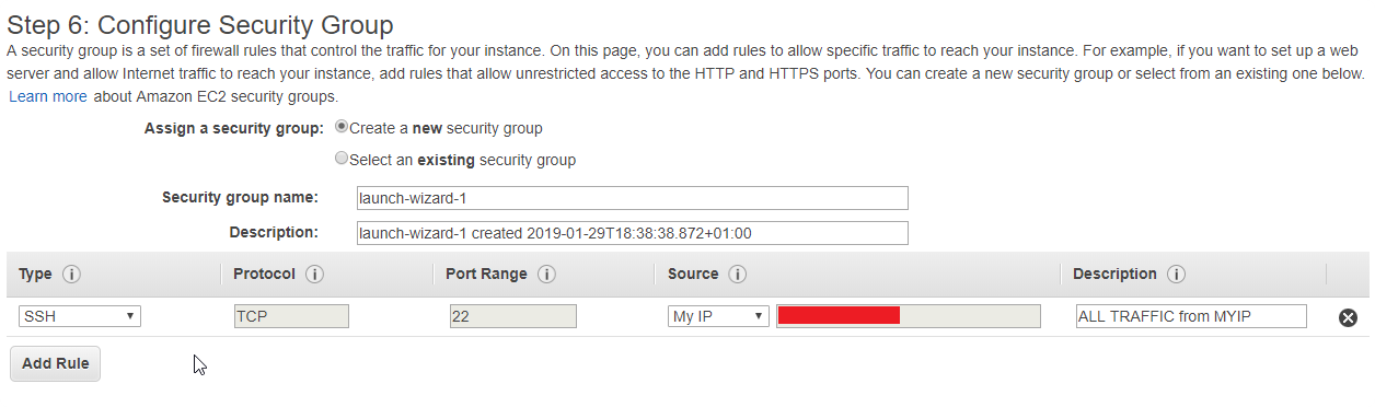
In Configure securiity Group, add your IP to allow from your IP allow to connect (it can be only SSH or All traffic if you want), and click next

1548792681361

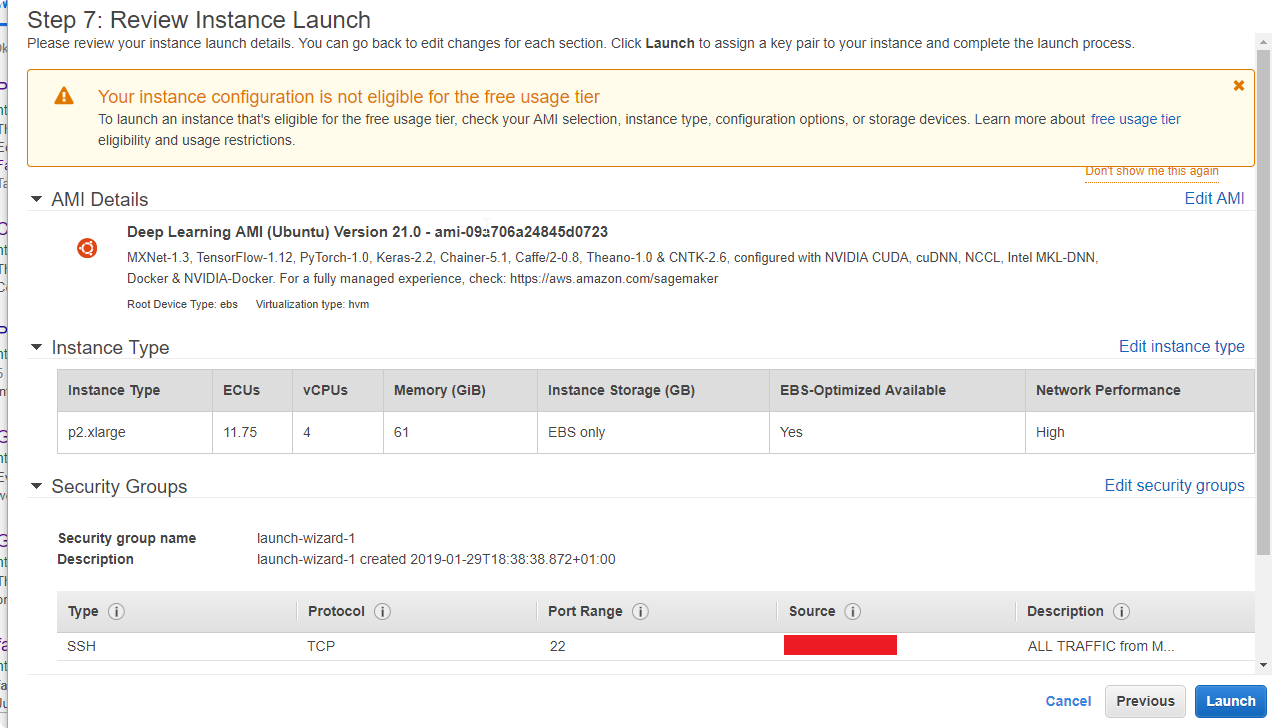
You will see that your network is not eligible for the free usage tier, click Launch.

1548792728048

Now you need to create your key pair to login into your instance. If you create one you can use the same, but first:

Choose name, and click Download Key Pair, and store the key in the safe place.

1548783776548

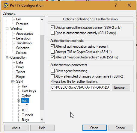
If you are using putty.exe, you need to divide your key into private and public key.

Download the puttygen.exe from the https://www.chiark.greenend.org.uk/~sgtatham/putty/latest.html
Click load to load your private/public key: (choose All Files *.*)

1548783977245

1548783995980

Click Save private key

1548784064758

This will generate your private key (.ppk) to use in the putty.exe

If you loose your key

You will loose your access to the server

Click view Instances

1548792807620

On the instance you can now login with the putty.exe

In a connection\SSH\Auth browse your private key (.ppk)

1548784332519

In the session write your IP

1548792569401

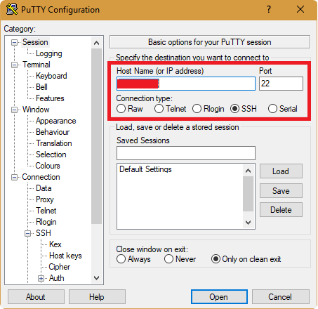
Login as ubuntu
update your libralies

conda install -c fastai fastai

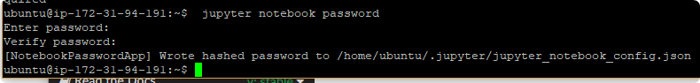
Setup password for your notebook

 jupyter notebook password

1548784862543

Run jupyter notebook

ipython notebook --no-browser --port=8002

Start tunneling to get to your notebook from the local webbrowser (-i is your downloaded .pem file from the Amazon AWS instance)

ssh -N -f -L localhost:8002:localhost:8002 ubuntu@__IP__ADRESS__ -i fastai-01.pem

got to the webpage: http://localhost:8002

1548785475325

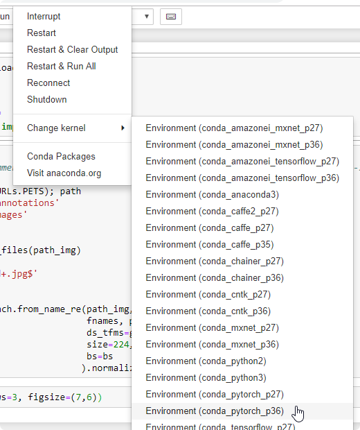
Verify you choose kernel: pytorch36

1548786200488

Verify library for fastai

from fastai import*
from fastai.vision import *

You will get the error about dataclasses. You need to install them

1548785884823

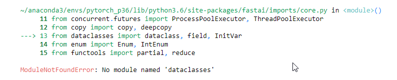
!pip install dataclasses

Verify download data:

bs = 64
# bs = 16   # uncomment this line if you run out of memory even after clicking Kernel->Restart

path = untar_data(URLs.PETS); path
path_anno = path/'annotations'
path_img = path/'images'


fnames = get_image_files(path_img)
np.random.seed(2)
pat = r'/([^/]+)_\d+.jpg$'


data = ImageDataBunch.from_name_re(path_img, 
                                   fnames, pat, 
                                   ds_tfms=get_transforms(), 
                                   size=224, 
                                   bs=bs
                                  ).normalize(imagenet_stats)

data.show_batch(rows=3, figsize=(7,6))

1548786238799

Error while loading data

Sometimes you will get the error:

RecursionError: maximum recursion depth exceeded while calling a Python object

You need to increase limit of the recursion:

import sys; sys.setrecursionlimit(10000) lub więcej, 100k

Verify creating model

print(data.classes)
#len(data.classes),data.c

learn = create_cnn(data, models.resnet34, metrics=error_rate)
print(learn.model)

Verify calculating epochs.

learn.fit_one_cycle(1)
interp = ClassificationInterpretation.from_learner(learn)
losses,idxs = interp.top_losses()


interp.plot_top_losses(9, figsize=(15,11))

1548786340529

1548786462857

Stop your instance after you finish working (or Terminate to remove the whole instance)

1548792872371

Remember to stop your instance

If you don’t do this Amazon will charge you for every hour of using your instance. If You only Stop your instance, Amazon will charge you for ELASTIC BLOCK STORE (Free Tier allow you to have maximum 30GB and p2.xlarge has 75GB) but the cost is much less than running machine (about 5 dollars per month).

installation / Google Cloud

Google cloud also is not a free option, but at the beginining you’ve got 300$ to use in your computer. It is enough to run a machine and go through all courses in the fast.ai library. First think you need to do is to create an account at https://cloud.google.com/.

Free credits are not eligible to run GPU machine, that’s why you need post a ticket to give you permission for GPU machine.

On your console https://console.cloud.google.com, in the IAM & Admin go to Quotas.

1551261621298

Filter metrics to GPUs (all regions)

1551261729127

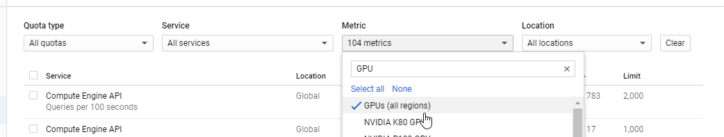
Click on the Compute Enginge API, and create new Quota.

1551261828322

Set up new limit to 1.

1551261869250

Wait for acceptance of your ticket. It could take couple hours, or even couple days.

1551261929324

When you have new limit, time to create a new instance. The best option is to create your instance by console. Install gcloud going trhough the instructions: https://cloud.google.com/sdk/docs/quickstarts

A lot of errors

I’ve got a lot of errors during installation on Windows 10. Most of them I resolved by restarting a system.

Now create your machine:

Windows command GPU

gcloud compute instances create "my-instance-01" --zone="us-west2-b" --image-family="pytorch-latest-gpu" --image-project=deeplearning-platform-release --maintenance-policy=TERMINATE --accelerator="type=nvidia-tesla-p4,count=1" --machine-type="n1-highmem-8" --boot-disk-size=200GB --metadata="install-nvidia-driver=True" --preemptible

WIndows command CPU

gcloud compute instances create "my-instance-01" --zone="us-west2-b" --image-family="pytorch-latest-cpu" --image-project=deeplearning-platform-release --maintenance-policy=TERMINATE  --machine-type="n1-highmem-8" --boot-disk-size=200GB --metadata="install-nvidia-driver=True" --preemptible

Bash/Linux:

export IMAGE_FAMILY="pytorch-latest-gpu" # or "pytorch-latest-cpu" for non-GPU instances
export ZONE="us-west2-b" # budget: "us-west1-b"
export INSTANCE_NAME="my-fastai-instance"
export INSTANCE_TYPE="n1-highmem-8" # budget: "n1-highmem-4"

# budget: 'type=nvidia-tesla-k80,count=1'
gcloud compute instances create $INSTANCE_NAME \
        --zone=$ZONE \
        --image-family=$IMAGE_FAMILY \
        --image-project=deeplearning-platform-release \
        --maintenance-policy=TERMINATE \
        --accelerator="type=nvidia-tesla-p4,count=1" \
        --machine-type=$INSTANCE_TYPE \
        --boot-disk-size=200GB \
        --metadata="install-nvidia-driver=True" \
        --preemptible

1551262933905

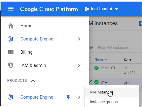
You should also see your instance in the google console. https://console.cloud.google.com

1551263023358

1551263120582

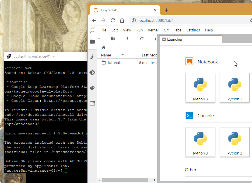
Now you can login to your jupyter notebook. This will forward a jupyter port 8080 to your localhost port.

gcloud compute ssh jupyter@my-instance-01 -- -L 8080:localhost:8080

gcloud compute ssh refuses connection (return code 255)

When I first try to login to the ssh I’ve got error 255. For this recreate your internal routing. more

gcloud compute routes list

gcloud compute routes create default-internet \
--destination-range 0.0.0.0/0 \
--next-hop-gateway default-internet-gateway

1551263348669

Update to the latest version

pip install fastai --upgrade

Create new notebook and run. (this version has already installed fastai)

from fastai import*
from fastai.vision import *
print(__version__)

bs = 64
# bs = 16   # uncomment this line if you run out of memory even after clicking Kernel->Restart

path = untar_data(URLs.PETS); path
path_anno = path/'annotations'
path_img = path/'images'


fnames = get_image_files(path_img)
np.random.seed(2)
pat = r'/([^/]+)_\d+.jpg$'


data = ImageDataBunch.from_name_re(path_img, 
                                   fnames, pat, 
                                   ds_tfms=get_transforms(), 
                                   size=224, 
                                   bs=bs
                                  ).normalize(imagenet_stats)

data.show_batch(rows=3, figsize=(7,6))

1551263919741

print(data.classes)
#len(data.classes),data.c

learn = create_cnn(data, models.resnet34, metrics=error_rate)
print(learn.model)

learn.fit_one_cycle(1)
interp = ClassificationInterpretation.from_learner(learn)
losses,idxs = interp.top_losses()


interp.plot_top_losses(9, figsize=(15,11))

1551264505006

Stop your instance

Remember to stop your instance on the console when you finish your work.

fast.ai / Help functions

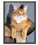
open_image()

Open single image,

im = open_image('images/Maine_Coon_97.jpg')

1549698053830

open_mask(fn)

Open mask by the function fn., that returns mask image file.

mask = open_mask(get_y_fn(img_f))
mask.show(figsize=(5,5), alpha=1)

1550779832997

.show()

Show image in the output.

im = open_image('images/Maine_Coon_97.jpg')
im.show(title='Title of the image')

1549698531867

.apply_tfms()

Apply transformation for the image and return new image.

im.apply_tfms(get_transforms()[0][3]).show()

1549736278158

ImageCleaner

Displays images for relabeling or deletion and saves changes in path.

from fastai.widgets import *

ds, idxs = DatasetFormatter().from_toplosses(learn, ds_type=DatasetType.Valid)
ImageCleaner(ds, idxs, path)

1550257534536

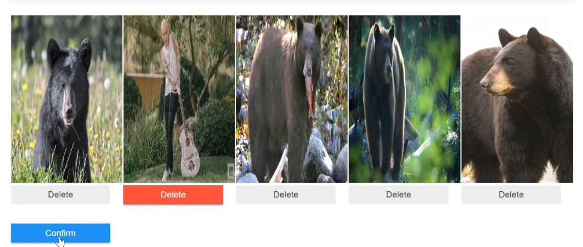
ImageCleaner doesn’t work on Google Colab

For this situation you need to delete files by yourself, or use Jupyter Notebook.

.show_heatmap()

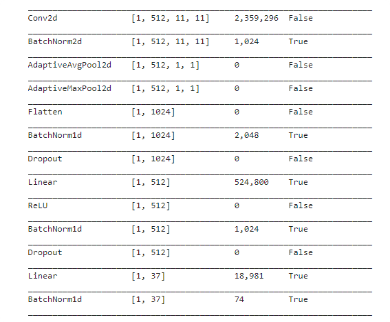
Pytorch alows you to hook the layer and store some information before. In the resnet34 if you look at the last layer you will find that last linea [1,37] is your layer for classification (cat/dogs breeds), previous layers are also flat layers with classification [512], this is the end of resnet34 model.

We have two groups of layers learn.model[0], and learn.model[1]. We can get first layer with the last Conv2dlayer, and BatchNorm2d that size is [1,512,11,11] , and usign hook_output to get what is stored in the output for that category (preds[0,int(cat)].backward()), next we get this information from the hook_a.stored[0].cpu() variable, and show the heatmap.

1552590896874

def show_heatmap(learn,x,y):
    m = learn.model.eval(); # set mode to evaluation mode
    xb,_ = learn.data.one_item(x)
    
    
    xb_im = Image(data.denorm(xb)[0]);
    
    
    xb = xb.cuda()
    
    print(xb.shape)
    
    from fastai.callbacks.hooks import hook_output
    def hooked_backward(cat=y):
        with hook_output(m[0]) as hook_a: 
            with hook_output(m[0], grad=True) as hook_g:
                # print(m[0])
                preds = m(xb)
                # print(preds.shape)
                preds[0,int(cat)].backward()
        print(hook_a.stored.shape)
        return hook_a,hook_g
    
    hook_a,hook_g = hooked_backward(y);
    acts  = hook_a.stored[0].cpu()
    avg_acts = acts.mean(0)
    
    print(acts.shape,avg_acts.shape)
    
    def show_heatmap(hm):
        _,ax = plt.subplots()
        xb_im.show(ax)
        _,width,height = xb_im.shape
        ax.imshow(hm, 
                  alpha=0.6, extent=(0,width,height,0),
                  interpolation='bilinear', cmap='magma');
        
    show_heatmap(avg_acts)

x,y = data.train_ds[5004]
show_heatmap(learn,x,y)

1552593708692

1552593695073

Another layer

Let’s now change m[0] to m[0][1]. This is a first layer of your network (after BatchNorm2d). What you can see that first layer regnozie edges of the pet.

1552594605148

fast.ai / Data

Before we put our data into learner we need to load them, and fast.ai gat a whole class that will divide your data into train, test , and validation, prepare some data augmentation so you don’t have to do it by yoursef

Basic functions

Name	Description
`data.c`	number of classes
`data.classes`	list of classes
`data.train_ds`	Train Dataset
`data.valid_ds`	Validation dataset
`data.test_ds`	Test dataset
`data.batch_size`	batch size
`data.dl(ds_type=DatasetType.Valid)`	Return data loader, (example: `ds.dl(DatasetType.Valid)`)
`data.one_item(item)`	Get `item` into a batch
`data.one_batch()`	Get one batch of from the DataBunch. Returns `x,y` with size of the `batch_size` (if `bs=128` then there is a list of 128 elements).

ImageDataBunch

Class that as an input have images.

parameter	description
`path`	folder path to the directory of images
`ds_tfms`	List of transformation for images
`size`	The size of the image as input for data (`width`and `height`for the image are the same). If the image is greater than will be cropped.

ImageDataBunch / from_folder

Load data that are prepared in the folder structure. train, test , valid

1549650957873

data = ImageDataBunch.from_folder(path, ds_tfms=get_transforms(), size=24)

1549650578727

ImageDataBunch / from_csv

When you’ve got a .csv file with filenmaes and classes

data = ImageDataBunch.from_csv(path, ds_tfms=get_transforms(), size=28)

1549651318454

1549651350934

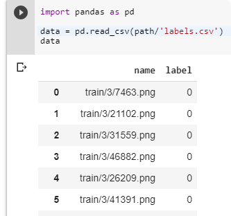
ImageDataBunch / from_df

Get data from loaded DataFrame

df = pd.read_csv(path/'labels.csv')
data = ImageDataBunch.from_df(path, df, ds_tfms=tfms, size=24)

[0,1]

ImageDataBunch / from_name_re

Get data from regular expression in the file name. regexr

1549652416468

pat = r"/(\d)/\d+\.png$"
data = ImageDataBunch.from_name_re(path, fnames, pat=pat, ds_tfms=get_transforms(), size=24)

['3', '7']

ImageDataBunch / from_name_func

data = ImageDataBunch.from_name_func(
    path, 
    fnames, 
    ds_tfms=get_transforms(), 
    size=24,
    label_func = lambda x: '3' if '/3/' in str(x) else '7')

['3', '7']

ImageDataBunch / from_list

Get Image data from the list that contains list of classes for each file in fnames.

labels = [('3' if '/3/' in str(x) else '7') for x in fnames]


data = ImageDataBunch.from_lists(path,
                                 fnames, 
                                 labels=labels, 
                                 ds_tfms=get_transforms(), 
                                 size=24)

['3', '7']

DataBunch / Own Item List

Usually you have a lot of datasets with a lot of different type of data, folder structure, etc… It is impossible to write all possible combinations to write your own DataBunch for calculation, that’s why you can step by step put different function on each step of your dataset.

No	Step	Description
1.	`DataType`	Define what is your DataSource, and what is the output
2.	`from_*`	Define how to get the input data (files, dataframes, csv)
3.	`split`	How to split your data for training, validation and test
4.	`label_*`	How to label your data, output y. Returns DataSet.
5.	`Transforms`	List of transformations for your input data
6.	`databunch(bs=*)`	Convert to `DataBunch`class
7.	`normalize()`	Optional step for DataBunch to normalize input.

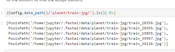
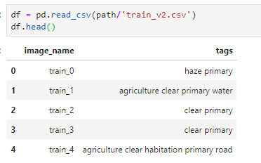
Examples 1/ Planet Data

We’ve got all files in one folder, without dividing into train and validation.

1550778286094

1550778228993



np.random.seed(42)
data = (ImageItemList
       .from_csv(path,
                 'train_v2.csv', 
                 folder='train-jpg', 
                 suffix='.jpg')
       .random_split_by_pct(0.2)
       .label_from_df(label_delim=' '))
	   .transform(tfms, size=128)
       .databunch(bs=16)
       .normalize(imagenet_stats))

We setup random value in the begining to get the same validation, and training set each time.
The Input is Image and output is list of categories, that’s why we use ImageItemList
The labels are form .csv file, the first column has image filename (default cols=0), and the file is train_v2.csv in the path. Folder for images is train-jpg, and after read the image name add suffix .jpg.
Because there is no split, we add random split 0.2
Labels are in the 1st column (default cols=1), with space delimeter label_delim
We add default transforms tfms, with flip_vert=True, because this are satelite images.
Create DataBunch, with bs=16.
We normalize images with imagenet_stats

Example 2 / IMDB DataBase

1550778883858

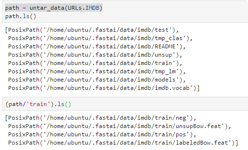
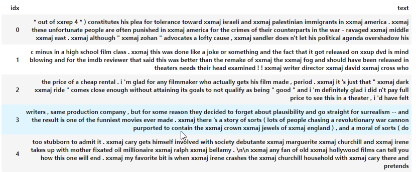
data_lm = (TextList.from_folder(path)
           #Inputs: all the text files in path
            .filter_by_folder(include=['train', 'test', 'unsup']) 
           #We may have other temp folders that contain text files so we only keep what's in train and test
            .random_split_by_pct(0.1)
           #We randomly split and keep 10% (10,000 reviews) for validation
            .label_for_lm()           
           #We want to do a language model so we label accordingly
            .databunch(bs=bs))

1550779135552

DataBunch / 1. DataType more

Class	Description
`CategoryList`	for labels and classification
`MultiCategoryList`	for labels in a multi classification problem
`FloatList`	for float labels in a regression problem
`ImageItemList`	for data that are images
`SegmentationItemList`	like `ImageItemList`but will default labels to `SegmentationLabelList`
`SegmentationLabelList`	for segmentation mask
`ObjectItemlist`	like `ImageItemList`but will default labels to `ObjectLabelList`
`PointsItemList`	for points (of the type `ImagePoints`)
`ImageList`	for image to image tasks
`TextList`	for text date
`TabularList`	for tabular data
`CollabList`	for collaborative filtering

DataBunch / 2. from_

function	Description
`from_folder(path)`	From folder defined in `path`more
`from_df(path, df)`	From DataFrame (`df`)
`from_csv(path,csv_name)`	Create ItemList from `.csv` file,

DataBunch / 3. split

How to split your data for training, validation and test.

function	Description
`no_split`	No split data between `train` and `val` (empty `validation set`)
`random_split_by_pct(valid_pct=0.2)`	Split by random value
`split_by_files(valid_names)`	Split by list of files for validation
`split_by_fname_file(fname,path)`	Split by list of files in the `fname`file.
`split_by_folder(train='train', valid='valid')`	Split by the folder name
`split_by_idx(valid_idx)`	Split by list of indexes of `valid_idx`
`split_by_idxs(train_idx,valid_idx)`	Split by list of indexes of `train_idx`, `valid_idx`
`split_by_list(train,valid)`	Split by list for `train`, and `valid`
`split_by_vavlid_func(func)`	Split by the function that return True if it is for `valido .`
`split_from_df(col)`	Split the data from `col` in the DataFrom

DataBunch / 4.label

Define the output for items (grand truth)

Name	Description
`label_empty()`	`EmptyLabel` for each item
`label_from_list(labels)`	Label from the list of labels
`label_from_df(cols=1)`	Set label as column in the dataframe
`label_const(const=0)`	Set label as value
`label_from_folder()`	Get label from the parent folder of the file (e.g. `cars\train\porshe\img_001.jpg`, tha label will be `porche`)
`label_from_func(func)`	Get label from the function
`label_from_re(pat)`	Get label from pattern
`label_for_lm()`	Labers are from Language Model

DataBunch / 5. Transforms more

Add list of transforms like Data augmentation

Parameter	Description
`tmfs`	List of random transformation
`size`	size of the image `(224,224)` or `224` if it’s square
`resize_method`	Type of resize: `ResizeMethod.CROP`
	`ResizeMethod.CROP` - resize so that the image fits in the desired canvas on its smaller side and crop
	`ResizeMethod.PAD` - resize so that the image fits in the desired canvas on its bigger side and crop
	`ResizeMethod.SQUISH` - resize theimage by squishing it in the desired canvas
	`ResizeMethod.NO` - doesn't resize the image
`padding_mode`	Padding mode
	`zeros` - fill with zeros
	`border` -fill with values from border pixel
	`reflection`- fill with reflection

.transform(tfms)

data = (ImageList.from_folder(path, 
                      convert_mode='L'
                     ).split_by_folder()
                      .label_from_folder()
                      .transform(tfms=get_transforms(), 
                                 size=(224,224), 
                                 padding_mode='border',
                                 resize_method=ResizeMethod.PAD)
                      .databunch(bs=64, num_workers=4).normalize())

1554552160493

DataBunch / 6. Dataunch

Convert to DataBunch. The difference from DataSet is that DataBunch divide data into train, valid, and test DataSet.

.databunch(bs=64)

Function	Description
`.show_batch(rows=5,ds_type=DatasetType.Train)`	Show in the result example images `ds_type=[DatasetType.Train, DatasetType.Test, DatasetType.Valid,Single, DatasetType.Fix]`
`.dl(ds_type)`	Returns `DeviceDataLoader`
`.c`	Return count of classes
`.classes`	List of classes
`.train_ds`, `train_dl`	Return train DataSet, or train DataLoader. First value is input, and second value is output.(e.g. `data.train_ds[0]`): `(Image (3, 128, 128), MultiCategory haze;primary)`
`valid_ds`, `valid_dl`	Valid DataSet, Valid DataLoader
`test_ds`, `test_dl`	Test DataSet, Test DataLoader

.normalize()

Normalize data based on the mean and standard devation of the image using the Standard Score ((x-mean)/std). For the image you normalize value for each channel separetely (R,G,B). If you download images from standard sources you can use predefined statistics. Otherwise use batch_stats() that returns statistics for your images.

cifar_stats = ([0.491, 0.482, 0.447], [0.247, 0.243, 0.261])
imagenet_stats = ([0.485, 0.456, 0.406], [0.229, 0.224, 0.225])
mnist_stats = ([0.15]*3, [0.15]*3)

data = ImageDataBunch.from_name_re(
    path_img, 
    fnames, 
    pat, 
    ds_tfms=get_transforms(), 
    size=224, bs=bs
)

data = data.normalize(data.batch_stats())

#or data = data.normalize(imagenet_stats)

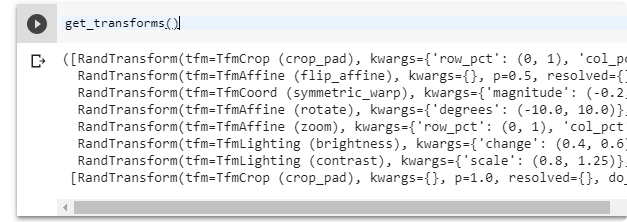
fast.ai / Data augmentation more

Group of functions that changes your data without changing the meaning of the data. Usefull to test your model when you want to add some data augmentation. For example little zoom on the image, flip the image, rotate in a small range).

get_transforms() source

Return list of transforms for the image that can be used in the ImageDataBunch as a df_tfms parameter. The list is divided into transformation for train and validation

parameter	description
`do_flip`	Image can be flipped
`flip_vert`	Image can be flipped vertically (like satelite images or images from top)
`max_rotate`	maximum rotation of the image (default: `10`)
`max_zoom`	maximum zoom of the image (default: `1.1`)
`max_lighting`	maximum lighting of the image (default: `0.2`)
`max_warp`	maximum warp of the image (default: `0.2`)
`p_affine`	the probability that each affine transform and symmetric warp is applied
`p_lighting`	the probability that each lighting transform is applied
`xtra_tfms`	a list of additional transforms

1549719418642

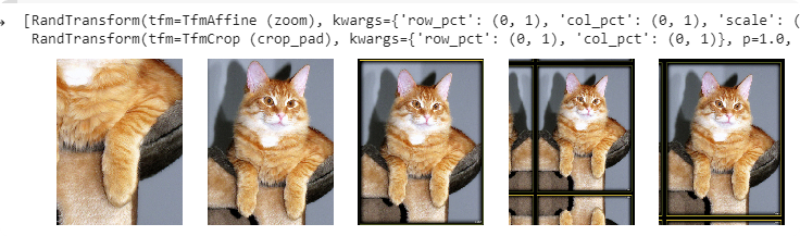
zoom crop() more

Randomly zoom and/or crop

parameter	description
`scale`	Decimal or range of decimals to zoom the image
`do_rand`	if true, transform is randomized
`p`	probability to apply the zzom

tsfms = zoom_crop(scale=(0.75, 2), do_rand=True)

1549721099158

rand_resize_crop()

Randomly resize and crop the image.

parameter	description
`size`	Final size of the image
`max_scale`	Zoom the image to a arandom scal up to this
`ratios`	Range of rations in which a new one will be randomly picked

tfms = [rand_resize_crop(224)]

1549721362837

List of transforms

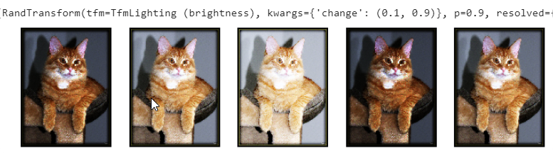
brightness() more

Apply change in brightness of image. (0 - black, 0.5 no change, 0.9 - bright)

tfms = [brightness(change=(0.1,0.9),p=0.9)]

1549722249727

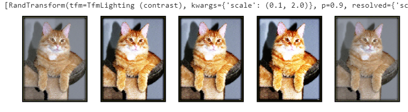
contrast more

Apply scale to contrast of the image. (0 - grey, >1 - super contrast, 1.0 - original image)

tfms = [contrast(scale=(0.1,2.0),p=0.9)]

1549722744720

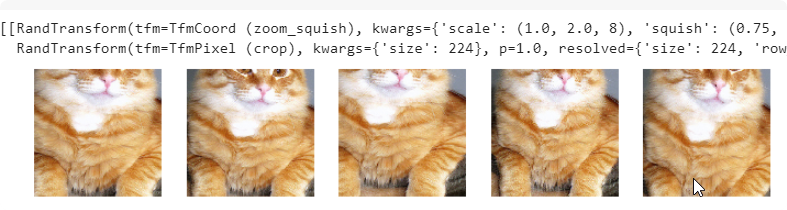
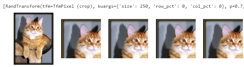
crop more

Crop the image with the size and return image with the new size.row_pct and col_pct are the position of the left/top corner.

tfms = [crop(size=250, row_pct=0,col_pct=0,p=0.7)]

1549723001104

crop pad more

Like crop, but if the final image is biggar it will also add padding to the image.

crop_pad(im, int(size), 'zeros', 0.,0.)

1549730189408

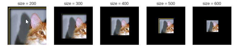
Why there is no effect in crop_pad on `apply_tfms`

crop_pad is used but on an image that was resized so that its lower dimension is equal to the size you pass.* source

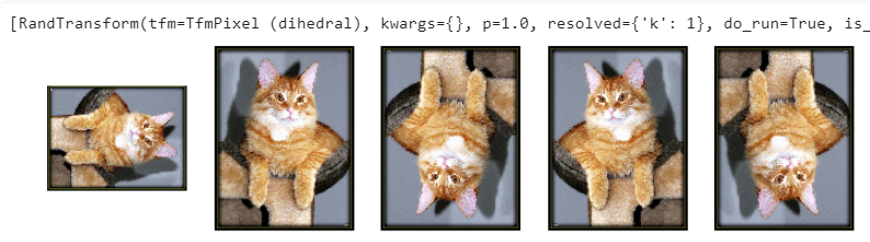
dihedralmore

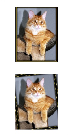
Randomly flip and apply rotation of a multiple of 90 degrees.

If the target is an ImagePoints, or an ImageBBox use dihedral_affine function.

tfms = [dihedral()]

1549731670616

for k, ax in enumerate(axs.flatten()):
    dihedral(im, k).show(ax=ax, title=f'k={k}')

1549731840065

flip lrmore

Randomly flip horizontaly.

If the target is an ImagePoints, or an ImageBBox use ``flip_affine`function.

tfms = [flip_lr(p=0.5)]

1549732187896

jitter more

Changes pixels randomly replacing them with pixels from the neighorbhood. magnitude parameter is used to get information how far the neighborhood extends.

tfms = [jitter(magnitude=(-0.05,0.05))]

1549732538184

pad more

Apply padding to the image: (padding - size of padding )

mode=zeros : pads with zeros
mode=border: repeats the pixels at the border
mode=reflection: pads by taking the pixels symmetric to the border

tfms = [pad(padding=30,mode='zeros',p=0.5)]

1549732802157

perspective warp more

Apply perspective warping that show a different 3D perspective of the image.

tfms = [perspective_warp(magnitude=(0,1),p=0.9)]

1549733306310

symmetric_warp more

Apply symetric warp of magnitude.

tfms = [symmetric_warp(magnitude=(-0.2,0.2))]

1549733878458

cutout more

Cut out n_holes number of square holes at random location

tfms = [cutout(n_holes=(1,20))]

1549734050015

fast.ai / Learner

Basic Functions

Function	Description
`learn.save('filename')`	Save learner
`learn.load('filename')`	Load learner from the file
`learn.export()`	Export the learner as pickle file `export.pkl`
`learn = load_learner(path)`	load learner from the folder whith the exported file `export.pkl`
`learn.load_encoder('fine_tuned_enc')`	Load encoder
`learn.save_encoder('fit-tuned-enc')`	Save encoder
`learn.data`	`DataBunch` connected with learner
Collaborative filtering:
`learn.bias(arr,is_item)`	a bias vector for user or item, `learn.bias(['Star Wars (1977)'],True)`
`learn.weight(arr,is_item)`	a weight matrix for user or item, `learn.weight(['Star Wars (1977)'],True)`
`parameters()`	list of all parameters

Encoder is used in seq2seq more problem, by techinque called trasfer learning.

The encoder is essentially tasked with creating a mathematical representation of the language based on the task for predicting the next word.
A decoder is responsible for taking that representation and applying it to some problem (e.g., predicting the next word, understanding sentiment, etc…) source

.show_results()

Show the output of the learning with Ground Truth, and Predictions.

learn.show_results(rows=3, figsize=(8,9))

1550783391484

.predict()

predict the data

Parameter	Description
item	The item to predict

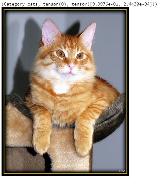
im = open_image(fnames[184])
learn.predict(im)

1549735528945

partial()

Partial is help function from Python, that can create a new function with different parameters. Normally accuracy_tresh get tresh=0.5, but with partial we can use this function with default tresh=0.2

acc_02 = partial(accuracy_thresh, thresh=0.2)
f_score = partial(fbeta, thresh=0.2)

learn = create_cnn(data, arch, metrics=[acc_02, f_score])

1550780654267

.to_fp16()

Normally precission is 32 bit, but you can downgrade this precission to 16bit. It can speed up yuor learning by 200%.

learn = learn.to_fp16()

Learner / cnn_learner()

Create a Learner object from the data object and model from the architecture.

Parameter	Description
`data`	DataBunch
`arch`	Architecture of the model
`metrics`	additional metrics to show during learning

data = ImageDataBunch.from_folder(path,
                                   ds_tfms=get_transforms(), 
                                   size=224, 
                                   bs=bs
                                  ).normalize(imagenet_stats)

learn = cnn_learner(data, models.resnet34, metrics=error_rate)

1549734500237

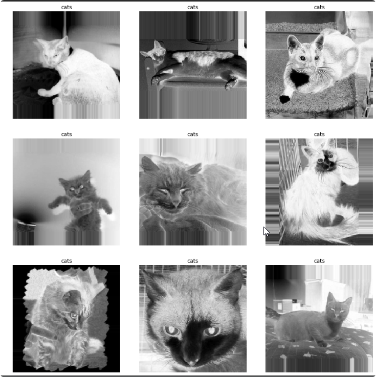
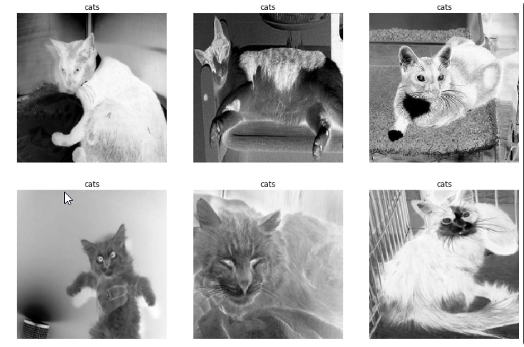
Example using ImageList and converts to Black&White

data = (ImageList.from_folder(path, 
                      convert_mode='L' # 'L', 'RGB', or 'CMYK'
                     ).split_by_folder()
                      .label_from_folder()
                      .transform(tfms=get_transforms(), 
                                 size=(224,224), 
                                 resize_method=ResizeMethod.SQUISH)
                      .databunch(bs=64, num_workers=4).normalize())
data.show_batch(3,3)

1554551513821

Learner / unet_learner() more more

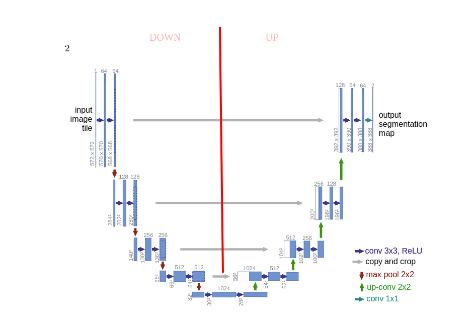
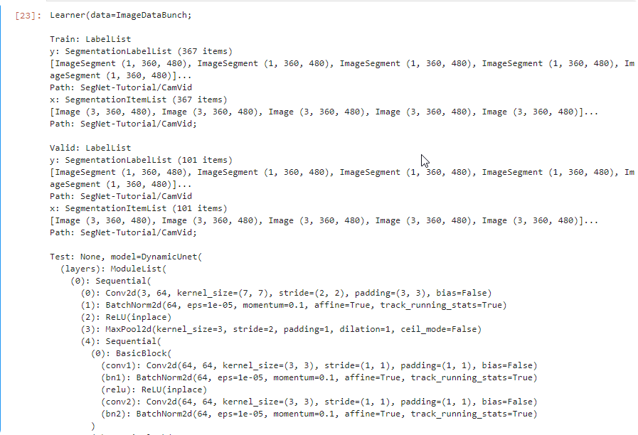
Create Unet architecture learner that converts image to image (mask). The suitable class that is used for DataBunch is SegmentationItemList (that is the same as ImageList).

Parameter	Description
`data`	DataBunch
`arch`	Architecture
`metrics`	List of metrics
`wd`	From Learner class `weight-decay` for regularization in Adam optimalization more
`bottle`	bottle flags if we use a bottleneck or not for that skip connection

learn = unet_learner(data, models.resnet34, metrics=metrics, wd=wd)

1550781130901

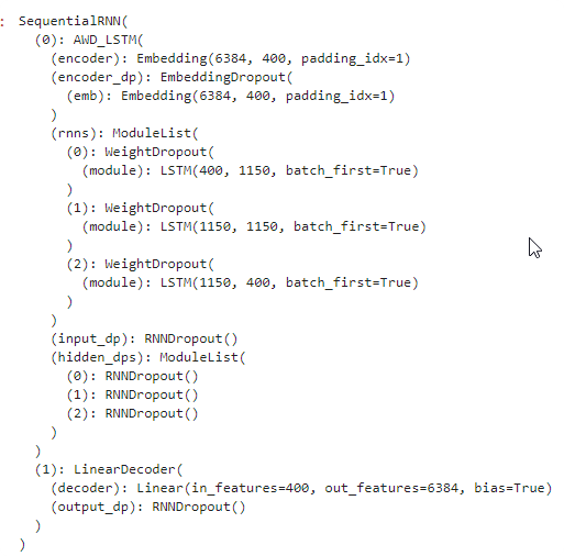
Learner / language_model_learner more

A learner for language model that predicts next word. Usuefull also as an encoder for text_classifier_learner

TextLMDataBunch - Text DataBunch for training a lanaguage model.

Parameter	Description
`data`	DataBunch
`arch`	Architecture (actually only `AWD_LSTM`)
`drop_mult`	`drop_mult` is applied to all the dropouts weights of the config. Parameter for `WeughtDropout` layer.
	TextLMDataBunch parameters:
`text_cols`	Text columns (`from_df` is the number of the column, default: 1)
`label_cols`	Label columns (`from_df` is the number of the column, default: 0)

1551290025513

twitter.csv

from fastai.text import *

path = './textdata'
file = 'twitter.csv'
data_lm = TextLMDataBunch.from_csv(path,file, text_cols='Name',label_cols='Style')

learn = language_model_learner(data_lm, AWD_LSTM, drop_mult=0.3)

1551290431811

Learner / text_classifier_learner

Learner to classify the text. It can be positive, or negative review, or the style of the text, or the emotion in the text. The TextClasDataBunch requires vocab value with vocabulary for the dataset.

A learner for language model that predicts next word. Usuefull also as an encoder for text_classifier_learner

Parameter	Description
`data`	DataBunch
`arch`	Architecture (actually only `AWD_LSTM`)
`drop_mult`	`drop_mult` is applied to all the dropouts weights of the config. Parameter for `WeughtDropout` layer.
	TextDataBunch parameters:
`path`	path of the file
`text_cols`	columns contain texts
`label_cols`	columns contain labels
`vocab`	vocabulary for text

data_clas = TextClasDataBunch.from_csv(path,file,
                                       text_cols='Name',
                                       label_cols='Style',
                                       vocab=data_lm.vocab)

learn = text_classifier_learner(data_clas, 
                                AWD_LSTM, 
                                drop_mult=0.5)

1551291317385

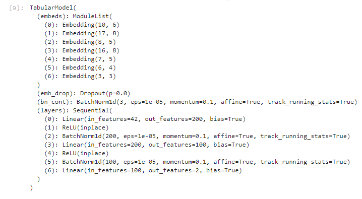
Learner / tabular_learner

Learner for the tabular data like XGBoost, to predict values based on columns in the DataFrame.

Parameter	Description
`data`	`TabularDataBunch`
`layers`	List of layers and size of each layer
`metrics`	additional metrics
TabularList parameters
`cat_names`	List of columns that are categories (also numbers like `day in month`)
`cont_names`	List of columns that are continuus numbers (like `cost`, `age`, `salary`)
`procs`	List of preprocessing for the input data
List of preprocessing classes:
`FillMissing`	Fill missing values, default using median more
`Categorify`	Categorize `cat_names`columns more
`Normalize`	Normalize input more

1551291408268

from fastai.tabular import *

procs = [FillMissing, Categorify, Normalize]
data = (TabularList.from_df(df, path=path, 
                            cat_names=cat_names, 
                            cont_names=cont_names, 
                            procs=procs)
                           .split_by_idx(list(range(800,1000)))
                           .label_from_df(cols=dep_var)
                           .add_test(test)
                           .databunch())

learn = tabular_learner(data, layers=[200,100], metrics=accuracy)

1551291709347

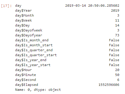
Tabular Learner / add_datepart

This function helps you to add additional information for date column. This is very helpful for your neural network, because it can recognize some seasonal changes(like on sunday people more often visit your store) . The list of columns that are added:

Year
Month
Week
Day
Dayofweek
Dayofyea
Is_month_end
Is_month_start
Is_quarter_end
Is_quarter_start
Is_year_end
Is_year_start
Hour (for time)
Minut
Second

Parameter	Description
`df`	DataFrame
`field_name`	Name of the field
`prefix`	prefix column
`drop`	drop original column?
`time`	add time columns

from fastai.tabular import *
import datetime


df = pd.DataFrame([datetime.datetime.now(),
             datetime.datetime.now() + datetime.timedelta(days=400)
             ], columns=['day'])


add_datepart(df,'day',prefix='day$',drop=False,time=True).iloc[0]

1552596629843

Train / fit

.fit()

function that train the model based on the train dataset.

Parameter	Description
epochs	Number of epochs
lr	Learning rate

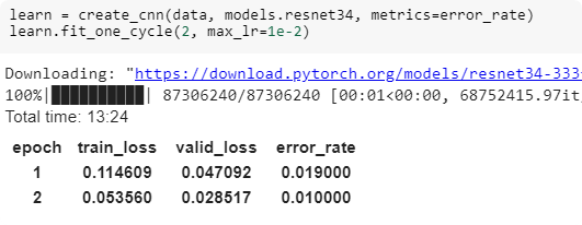
learn.fit(1,lr=1e-2)

1549735202902

.fit_one_cycle()

A better function to fit, that used 1cycle policy more more

learn.fit_one_cycle(1,max_lr=slice(3e-5,3e-3),moms=(0.95,0.85))

What’s the difference?:

In the fit you always go with the same learning rate through all epoch. In the fit_one_cycle you define maximum learnig rate. On each cycle the learning rate go through half of the iterations from the minimum learning rate to the defined maximum, and next half of the iterations go down to the minimum. On last couple of iterations the learning rate small decreasing.

1. We progressively increase our learning rate from lr_max/div_factor to lr_max and at the same time we progressively decrease our momentum from mom_max to mom_min.
2. We do the exact opposite: we progressively decrease our learning rate from lr_max to lr_max/div_factor and at the same time we progressively increase our momentum from mom_min to mom_max.
3. We further decrease our learning rate from lr_max/div_factor to lr_max/(div_factor x 100) and we keep momentum steady at mom_max.

Learning rates to use in a cycle

Parameter	Description
cyc_len	number of cycles
max_lr	maximum learning rate. We can use `slice(3e-5,3e-3)` to distribute learning rate between initial layers (first smaller value `3e-5`) to later layers (second higher value `3e-3`)
moms	`default: (0.95,0.85)` Momentum value. Momentum is intended to help speed the optimisation process through cases, to avoid getting stuck in the "shallow valleys" when gradient is close to 0. more (e.g. `moms=(0.95,0.85)` - momentum goes through the iterations like in the picture below )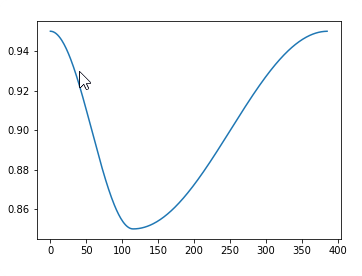

1549735023401

Improve

Name	Description
`unfreeze()`	Unfreeze entire model. `fit`, and `fit_one_cycle` will update weights on all layers.
`freeze()`	Freeze up to last layer.
`freeze_to(n=2)`	Freeze up to `n` layers. `fit` and `fit_one_cycle` will update weights on `n` last layers.

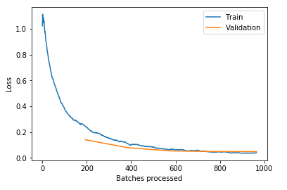
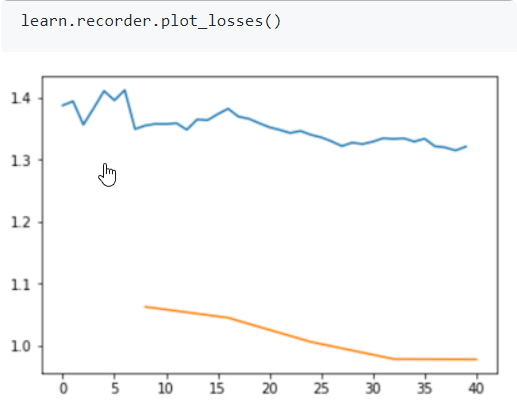
.recorder.plot_losses() more

Plot losses for the train and vaildation set. (after you call fit(), or fit_one_cycle())

learn.recorder.plot_losses()

1550170847911

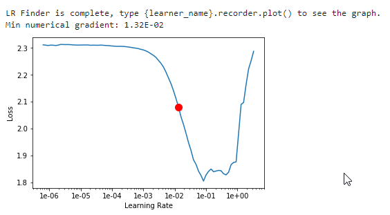
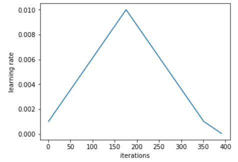
lr_find() more

Find best learning rate for a model. Determines how you update the weights or parameters.

learn.unfreeze()
learn.lr_find()

Parameter	Description
`start_lr`	start learning rate `float` number or `numpy array` (for example `learn.lr_find(np.array([1e-4,1e-3,1e-2]))`)
`end_lr`	The maximum learning rate to try.
`num_it`	Maximum number of iterations

learn.recorder.plot()

Plot learning rate and losses.

1550170981108

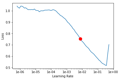
How to choose learning rate?

for learning rate you choose usualy two values that are distribute learning rate between layers. The first value 3e-5 you can find in the recorder.plot() and it is he strongest downward slope that's kind of sticking around for quite a while. more and for the top learning rate usualy choose 1e-4 or 3e-4, and it depends on you.

learn.fit_one_cycle(2, max_lr=slice(3e-5,3e-4))

Learning rate (LR) too high

What you get is much higher valid_loss than train_loss. You have to go back and create your neural net again and fit from scratch with a lower learning rate.

Total time: 00:13
epoch  train_loss  valid_loss  error_rate       
1      12.220007   1144188288.000000  0.765957    (00:13)

Learning rate (LR) too low

When your learning rate is too low your valid_loss will go down very slow, our error_rate go down but very slow. Try first show plot losses. If you have a model like that, train it some more or train it with a higher learning rate.

1550256445505

Total time: 00:57
epoch  train_loss  valid_loss  error_rate
1      1.030236    0.179226    0.028369    (00:14)
2      0.561508    0.055464    0.014184    (00:13)
3      0.396103    0.053801    0.014184    (00:13)
4      0.316883    0.050197    0.021277    (00:15)

Too few epochs

When you train in too few epochs, your train_loss is much higher than valid_loss. You can try more epochs, if it goes down very slow like in previous example, try highger learning rate.

Total time: 00:14
epoch  train_loss  valid_loss  error_rate
1      0.602823    0.119616    0.049645    (00:14)

Too many epochs

Too many epochs create something called "overfitting". Your error rate improves for a while and then starts getting worse again.

Any model that is trained correctly will always have train loss lower than validation loss.

33     0.189988    0.210684    0.065934    (00:09)
34     0.181293    0.214666    0.073260    (00:09)
35     0.184095    0.222575    0.073260    (00:09)
36     0.194615    0.229198    0.076923    (00:10)
37     0.186165    0.218206    0.075092    (00:09)
38     0.176623    0.207198    0.062271    (00:10)
39     0.166854    0.207256    0.065934    (00:10)
40     0.162692    0.206044    0.062271    (00:09)

fast.ai / Own Models

Learner

Instead of using prepared models, you can create your own one, and by class Learner use in the same way as other learners.

model = nn.Sequential(
    nn.Conv2d(in_channels=1, out_channels=8,kernel_size=3, stride=2, padding=1), # 14
    nn.BatchNorm2d(8),
    nn.ReLU(),
    nn.Conv2d(in_channels=8, out_channels=16,kernel_size=3, stride=2, padding=1), # 7
    nn.BatchNorm2d(16),
    nn.ReLU(),
    nn.Conv2d(in_channels=16, out_channels=32,kernel_size=3, stride=2, padding=1), # 4
    nn.BatchNorm2d(32),
    nn.ReLU(),
    nn.Conv2d(in_channels=32, out_channels=16,kernel_size=3, stride=2, padding=1), # 2
    nn.BatchNorm2d(16),
    nn.ReLU(),
    nn.Conv2d(in_channels=16, out_channels=10,kernel_size=3, stride=2, padding=1), # 1
    nn.BatchNorm2d(10),
    Flatten()     # remove (1,1) grid
)
learn = Learner(data, 
                model, 
                loss_func = nn.CrossEntropyLoss(), 
                metrics=accuracy)
print(learn.summary())

1554632305282

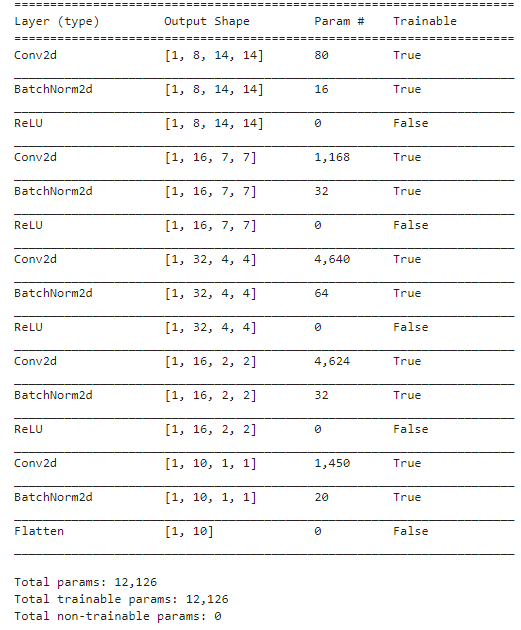
data.show_batch(rows=3, figsize=(5,5))

1554632326883

learn.lr_find(end_lr=100)
learn.recorder.plot()

1554632348629

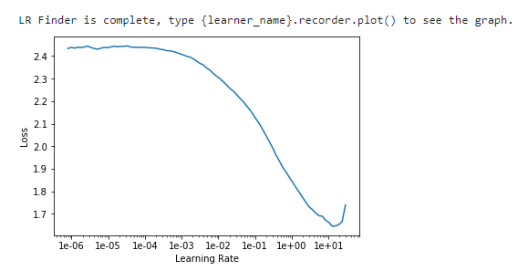
learn.fit_one_cycle(3, max_lr=0.1)

1554632377114

learn.predict(data.train_ds[0][0])

1554632400541

You can short your model with conv_layer function

model = nn.Sequential(
    conv_layer(1,8,ks=3,stride=2,padding=1)
#    nn.Conv2d(in_channels=1, out_channels=8,kernel_size=3, stride=2, padding=1), # 14
#    nn.BatchNorm2d(8),
#    nn.ReLU(),
    conv_layer(8,16,ks=3,stride=2,padding=1)
#    nn.Conv2d(in_channels=8, out_channels=16,kernel_size=3, stride=2, padding=1), # 7
#    nn.BatchNorm2d(16),
#    nn.ReLU(),
    conv_layer(16,32,ks=3,stride=2,padding=1)
#    nn.Conv2d(in_channels=16, out_channels=32,kernel_size=3, stride=2, padding=1), # 4
#    nn.BatchNorm2d(32),
#    nn.ReLU(),
    conv_layer(32,16,ks=3,stride=2,padding=1)
#    nn.Conv2d(in_channels=32, out_channels=16,kernel_size=3, stride=2, padding=1), # 2
#    nn.BatchNorm2d(16),
#    nn.ReLU(),
    nn.Conv2d(in_channels=16, out_channels=10,kernel_size=3, stride=2, padding=1), # 1
    nn.BatchNorm2d(10),
    Flatten()     # remove (1,1) grid
)

Reasidual Learning more

Adding more layers usually doesn’t improve model. If we create a 56-layer model it would be worse than 20-layer model.

1554633099049

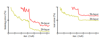
What would happende if we create something that skip

1554633275010

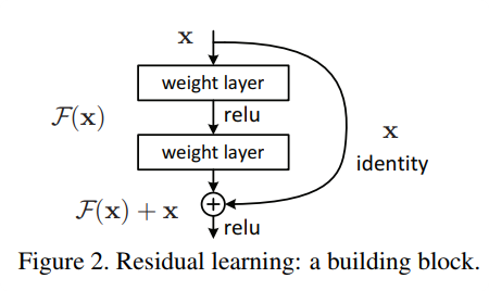
This is used in the ResNet network, that each layer is the ResNet Block.

class ResBlock(nn.Module):
    def __init__(self, nf):
        super().__init__()
        self.conv1 = conv_layer(nf,nf)
        self.conv2 = conv_layer(nf,nf)
        
    def forward(self, x): return x + self.conv2(self.conv1(x))

or you can use build in function res_bloc.

res_block(8)

1554636864336

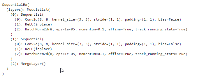
def conv2(ni,nf): return conv_layer(ni,nf,stride=2)
def conv_and_res(ni,nf): return nn.Sequential(conv2(ni, nf), res_block(nf))

model = nn.Sequential(
    conv_and_res(1, 8),
    conv_and_res(8, 16),
    conv_and_res(16, 32),
    conv_and_res(32, 16),
    conv2(16, 10),
    Flatten()
)

learn = Learner(data, 
                model, 
                loss_func = nn.CrossEntropyLoss(), 
                metrics=accuracy)
learn.fit_one_cycle(3, max_lr=0.1)

1554636957515

fast.ai / Examples

dog-cat example

download

from fastai import*
from fastai.vision import *

path = untar_data(URLs.DOGS);

!ls /root/.fastai/data/dogscats
!ls /root/.fastai/data/dogscats/train

1549483689248

Train model

Train the model based on the previous learned model: resnet34 with learning reate=0.01 and 2 cycles

bs = 64
data = ImageDataBunch.from_folder(path,
                                   ds_tfms=get_transforms(), 
                                   size=224, 
                                   bs=bs
                                  ).normalize(imagenet_stats)
learn = create_cnn(data, models.resnet34, metrics=error_rate)
learn.fit_one_cycle(2, max_lr=1e-2)

1549630231237

Most incorrect data

interp = ClassificationInterpretation.from_learner(learn)
# losses,idxs = interp.top_losses()
interp.plot_top_losses(9, figsize=(15,11))

1549630263523

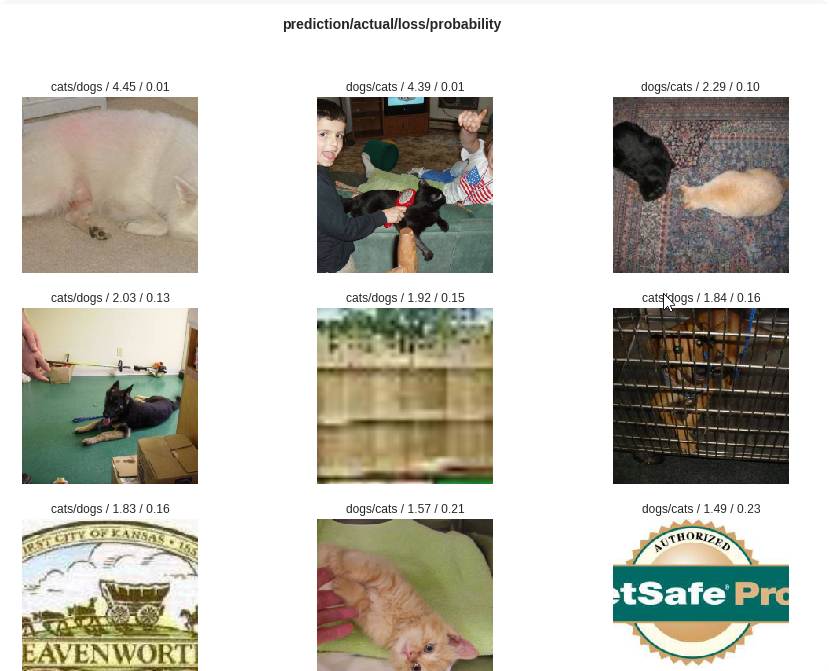
interp.plot_confusion_matrix()

1549630283099

Improve model

find better learn_fs

learn.lr_find()
learn.sched.plot()

1549630308144

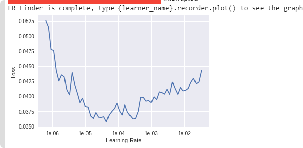
learn.unfreeze()
learn.fit_one_cycle(8, max_lr=slice(1e-5,1e-2))

1549630351231

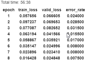
Our model val improve from 0.0100 to 0.007

interp.plot_confusion_matrix()

1549630404325

dogs/cats breeds example

This examples is more complicated that recognizing dogs and cats. It can also recognize 12 cat breeds and 25 dogs breeds. The whole core functions are the same as previous. The only difference is that now we use URLS.PETS to download data and ImageDataBunch.from_name_re.

Get data

from fastai.vision import *
from fastai.metrics import error_rate

path = untar_data(URLs.PETS);
path.ls()
(path/'images').ls()
path_img = path/'images';

1549484272998

1549484431215

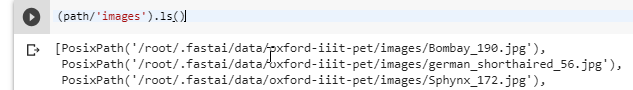
Get Data

fnames = get_image_files(path_img)
pat = r'/([^/]+)_\d+.jpg$'

data = ImageDataBunch.from_name_re(
    path_img, 
    fnames, 
    pat, 
    ds_tfms=get_transforms(), 
    size=224, bs=bs
).normalize(imagenet_stats)

print(data.classes)
data.show_batch(rows=4, figsize=(7,6))

['Abyssinian', 'Bengal', 'Birman', 'Bombay', 'British_Shorthair', 'Egyptian_Mau', 'Maine_Coon', 'Persian', 'Ragdoll', 'Russian_Blue', 'Siamese', 'Sphynx', 'american_bulldog', 'american_pit_bull_terrier', 'basset_hound', 'beagle', 'boxer', 'chihuahua', 'english_cocker_spaniel', 'english_setter', 'german_shorthaired', 'great_pyrenees', 'havanese', 'japanese_chin', 'keeshond', 'leonberger', 'miniature_pinscher', 'newfoundland', 'pomeranian', 'pug', 'saint_bernard', 'samoyed', 'scottish_terrier', 'shiba_inu', 'staffordshire_bull_terrier', 'wheaten_terrier', 'yorkshire_terrier']

1549630449518

Learn using resnet34

learn = create_cnn(data, models.resnet34, metrics=error_rate)
learn.fit_one_cycle(4)
learn.save('stage-1')

1549630532549

interp = ClassificationInterpretation.from_learner(learn)
interp.plot_top_losses(9, figsize=(15,11))

1549630635258

Most confused breeds

interp.most_confused(min_val=2)

[('Egyptian_Mau', 'Bengal', 11), ('american_pit_bull_terrier', 'staffordshire_bull_terrier', 7), ('British_Shorthair', 'Russian_Blue', 5), ('Persian', 'Ragdoll', 4), ('staffordshire_bull_terrier', 'american_pit_bull_terrier', 4), ('american_bulldog', 'staffordshire_bull_terrier', 3), ('beagle', 'basset_hound', 3), ('miniature_pinscher', 'chihuahua', 3)]

Find better learning rate

learn.lr_find()
learn.recorder.plot()

1549631049501

There is no point to train the whole network with a small value. Better is to define a small learning layer on the first layers and higher learning rate on the last layer and distribute other layers with values between.

learn.unfreeze()
learn.fit_one_cycle(2, max_lr=slice(1e-6,1e-4))

1549630793542

After we define the error rate drop to 0.06 which is a good value (better than human).

Resnet50

from fastai.vision import *
from fastai.metrics import error_rate

path = untar_data(URLs.PETS);
path_img = path/'images'
fnames = get_image_files(path_img)
pat = r'/([^/]+)_\d+.jpg$'

bs = 64

data = ImageDataBunch.from_name_re(
    path_img, 
    fnames, pat, 
    ds_tfms=get_transforms(),
    size=299, bs=bs//2).normalize(imagenet_stats)

learn = create_cnn(data, models.resnet50, metrics=error_rate)

learn.lr_find()
learn.recorder.plot()

learn.fit_one_cycle(8)
learn.save('stage-1-50')

1549631790524

1549631798510

learn.unfreeze()
learn.fit_one_cycle(3, max_lr=slice(1e-6,1e-4))

1549631818381

ISIC - Archive (Skin melanoma recognition)

ISIC archive contains plenty of skin images categorised and available for download from the webpage https://www.isic-archive.com. This is a good point to test fast.ai and verify the first fast.ai lesson for this list of images.

I’ve used the CurlWget to generate wget command that can be copied to the jupyter notebook and download the whole archive.

1549633920675

1549633967565

1549634016294

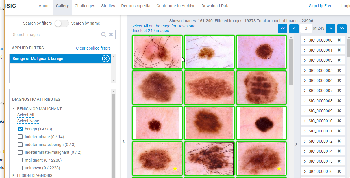
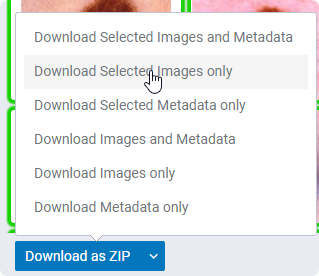
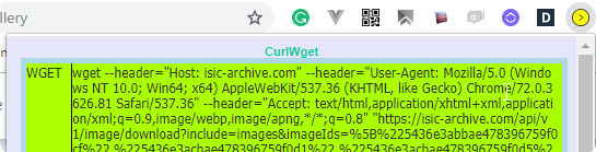
After you download first selected 240 images, and next selected 240 images for the bening.

#part 1 (240 images 1-3 pages)
!rm ISIC-images.zip
!wget ......
!unzip -o -q ISIC-images.zip -d isd/benign
!cp isd/benign/ISIC-images/**/*.jpg isd/benign

#part 2 (240 images 4-6 pages)
!rm ISIC-images.zip
!wget ...
!unzip -o -q ISIC-images.zip -d isd/benign
!mv isd/benign/ISIC-images/**/*.jpg isd/benign


#part 1 malignant
!rm ISIC-images.zip
!wget ...
!unzip -o -q ISIC-images.zip -d isd/malignant
!mv isd/malignant/ISIC-images/**/*.jpg isd/malignant

#part 2 (page 4-6 - 240 images)
!rm ISIC-images.zip
!wget ...
!unzip -o -q ISIC-images.zip -d isd/malignant
!mv isd/malignant/ISIC-images/**/*.jpg isd/malignant

Second option to download data

You can use a python library to download images https://github.com/GalAvineri/ISIC-Archive-Downloader .

!git clone https://github.com/GalAvineri/ISIC-Archive-Downloader.git
  
!mkdir isic
!mkdir isic/bening
!mkdir isic/malignant

!python "ISIC-Archive-Downloader/download_archive.py" --num-images 500  --filter benign --images-dir isic/bening
!python "ISIC-Archive-Downloader/download_archive.py" --num-images 500  --filter malignant --images-dir isic/malignant

1549636028509

1549636128365

Import libraries

I’ve used the recurse option to get also filenames from the subfolder.

from fastai import *
from fastai.vision import *
from fastai.metrics import error_rate
from pathlib import Path


bs = 64
#bs = 32   # uncomment this line if you run out of memory even after clicking Kernel->Restart

path = Path('./isic/')
fnames = get_image_files(path, recurse=True)

Then I can create the ImageDataBunch to prepare data to learn. I can filp vertical the images (get_transforms(filp_vert=True) ) because the image is not done from front but from the above. (like satelite images) and for recognition it doesn’t matter.

The example path is:

isic/bening/ISIC_000001.jpg

The regular expresssion is try to find regular expression.

r - means that text is regular expression
([a-zA-Z]+) - the name contains text and because they are in the first bracket they are used as a class for image recognition(bening or malignant)
ISIC_\d+.jpg - any file with the extension .jpg and name started as ISIC_ with the number \d+ after underline.
$ - this means that this that whole regex should be in the on of the name (like .jpg.jpg wouldn’t match the experession)

You can verify your regex on the page regexr.

1549645995061

pat = r"([a-zA-Z]+)/ISIC_\d+\.jpg$"

data = ImageDataBunch.from_name_re(path, 
                                   fnames, 
                                   pat=pat, 
                                   ds_tfms=get_transforms(flip_vert=True),  #FLIP VERTICAL 
                                   size=224).normalize(imagenet_stats)
print(data.classes)
data.show_batch(rows=3, figsize=(7,6))

1549635940232

Now we can try our first learn

learn = create_cnn(data, models.resnet34, metrics=error_rate)
learn.fit_one_cycle(4)
learn.save('stage-1')

1549636165565

This is not a very good result but we can try to find better learning rate. It shws that propably 1e-2 is the best to learn. This is one magnifi

learn.lr_find()
learn.recorder.plot()

1549636207163

learn.unfreeze()
learn.fit_one_cycle(8, max_lr=slice(1e-6,1e-2))

1549646496183

interp = ClassificationInterpretation.from_learner(learn)
interp.plot_confusion_matrix()

1549646581287

I go down with the 14% of error rate. This is not yet a good result, but for now enough to improvement in the future. Mostly the problem is with the skin that is consider as bening, but in real they are malignant.

Planet Amazon dataset

Planet Amazon DataSet is the DataSet of satellite images, that we can categorize with multiple labes for each image.

https://www.kaggle.com/c/planet-understanding-the-amazon-from-space

Download Data

from fastai.vision import *

path = Config.data_path()/'planet'
path.mkdir(parents=True, exist_ok=True)

!kaggle competitions download -c planet-understanding-the-amazon-from-space -f train-jpg.tar.7z -p {path} !kaggle competitions download -c planet-understanding-the-amazon-from-space -f train_v2.csv -p {path}  

!conda install -y -c haasad eidl7zip #install 7zip if not exist

!unzip -q -n {path}/train_v2.csv.zip -d {path}
!7za -bd -y -so x {path}/train-jpg.tar.7z | tar xf - -C {path}

Load Data

from fastai.vision import *

path = Config.data_path()/'planet'
df = pd.read_csv(path/'train_v2.csv')

tfms = get_transforms(flip_vert=True, max_lighting=0.1, max_zoom=1.05, max_warp=0.)


np.random.seed(42)
src = (ImageList
       .from_csv(path, 'train_v2.csv', folder='train-jpg', suffix='.jpg')
       .random_split_by_pct(0.2)
       .label_from_df(label_delim=' '))

data = (src
        .transform(tfms, size=128)
        .databunch(bs=16)
        .normalize(imagenet_stats))

data.show_batch(rows=3, figsize=(12,9))

1550781434208

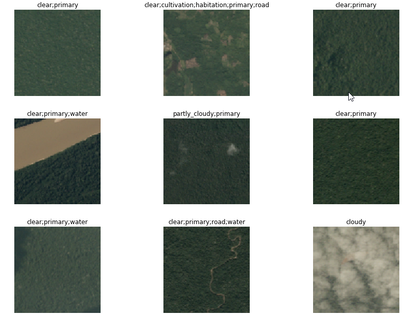
Load Learner

F-score is helpful for Kaggle competitions. Submission is for the F2-score, with bethaequal=2. (this is default for fbeta function)

1550781708755

1550781531925

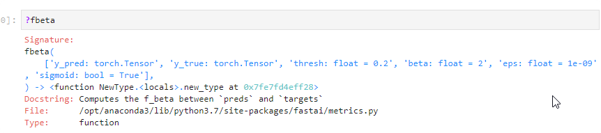
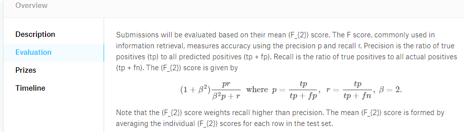
arch = models.resnet50

acc_02 = partial(accuracy_thresh, thresh=0.2)
f_score = partial(fbeta, thresh=0.2)

learn = create_cnn(data, arch, metrics=[acc_02, f_score])

Find learning rate

learn.lr_find()
learn.recorder.plot()

1550781750813

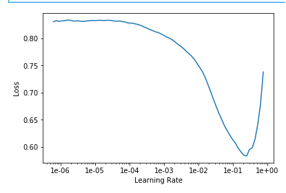
Learn Model

lr = 0.01
learn.fit_one_cycle(5, slice(lr))

1550781783734

Tune model

learn.unfreeze()
learn.lr_find()
learn.recorder.plot()

1550782018201

lr = 0.01
learn.fit_one_cycle(5, slice(1e-5, lr/5))
learn.save('stage-2-rn50')

1550781829671

We can resize the model to smaller images and retrain again.

learn.load('stage-2-rn50');

data = (src
        .transform(tfms, size=256)
        .databunch(bs=16)
        .normalize(imagenet_stats))

learn.data = data

learn.freeze()
learn.lr_find()
learn.recorder.plot()

1550782136754

lr=1e-2/2
learn.fit_one_cycle(5, slice(lr))

1550782161671

learn.unfreeze()
learn.fit_one_cycle(5, slice(1e-5, lr/5))
learn.recorder.plot_losses()
learn.save('stage-2-256-rn50')

1550782237657

1550782247706

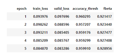
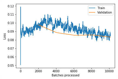
CamVid / mask Images

CamVid DataSet is huge dataset with images from camera in the car and mask that each pixel give some class. This is a classification for each pixel. The inptu is image, and the output is also image with classes instead of RGB.

http://mi.eng.cam.ac.uk/research/projects/VideoRec/CamVid/

Load Data

from fastai.vision import *
from fastai.callbacks.hooks import *

path = untar_data(URLs.CAMVID)
path_lbl = path/'labels'
path_img = path/'images'

fnames = get_image_files(path_img)
lbl_names = get_image_files(path_lbl)

path.ls()

1550782441540

We can load the image by open_image, and mask by open_mask. (x.stem is filename without extenstion, x.suffix is the extension). We can combine input file with the output by adding _P in the file name for path_lbl o directory.

1550782825543

img_f = fnames[0]
img = open_image(img_f)
img.show(figsize=(5,5))

get_y_fn = lambda x: path_lbl/f'{x.stem}_P{x.suffix}'
mask = open_mask(get_y_fn(img_f))
mask.show(figsize=(5,5), alpha=1)

1550782654727

1550782661576

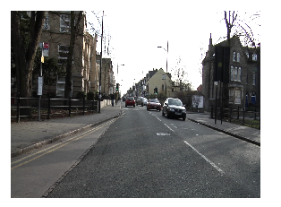
src_size = np.array(mask.shape[1:])
codes = np.loadtxt(path/'codes.txt', dtype=str);

Codes give us list of codes in the order. When in valudation set if pixel on the position x,y has value 0, this means that this is Animal,

1550782526202

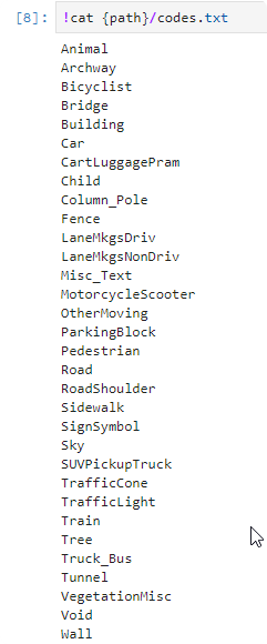
Create DataSet

First size of the DataSet is twice smaller than regular. This is called: "progressive resizing". The dataset learn faster and generalized better.

size = src_size//2
bs=4

src = (SegmentationItemList
       .from_folder(path_img)
       .split_by_fname_file('../valid.txt')
       .label_from_func(get_y_fn, classes=codes))

data = (src
        .transform(get_transforms(), size=size, tfm_y=True)
        .databunch(bs=bs)
        .normalize(imagenet_stats))

data.show_batch(5, figsize=(10,7),alpha=0.5)

For mask DataBunch, you can define alpha to set opacity for the mask. (1.0 - means you will not see image)

1550783072226

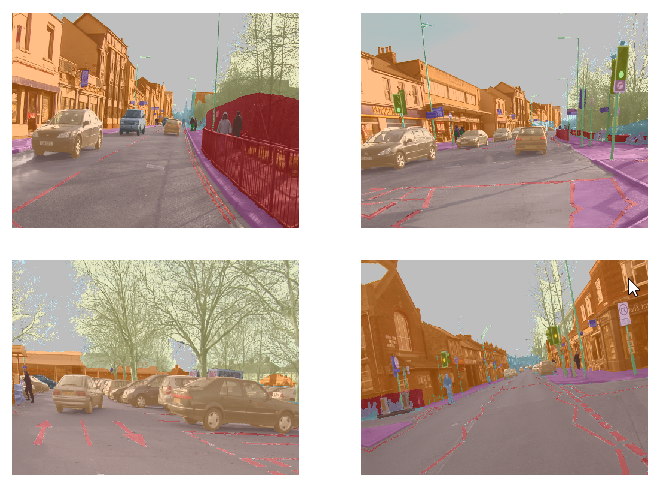
Create Model

We create our own accuracy, without void class for the image.

name2id = {v:k for k,v in enumerate(codes)}
void_code = name2id['Void']

def acc_camvid(input, target):
    target = target.squeeze(1)
    mask = target != void_code
    return (input.argmax(dim=1)[mask]==target[mask]).float().mean()

metrics=acc_camvid
wd=1e-2
learn = unet_learner(data, 
                     models.resnet34, 
                     metrics=metrics, 
                     wd=wd)

Find LR

lr_find(learn)
learn.recorder.plot()

1550783275635

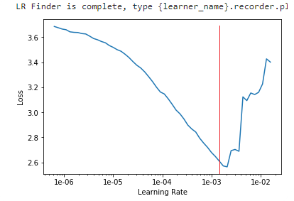
lr=3e-3
learn.fit_one_cycle(10, slice(lr), pct_start=0.9)
learn.save('stage-1')
learn.show_results(rows=3, figsize=(8,9))

1550783296270

1550783514365

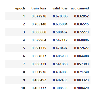
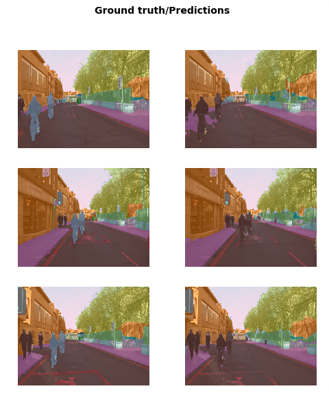
learn.unfreeze()
lrs = slice(lr/400,lr/4)
learn.fit_one_cycle(12, lrs, pct_start=0.8)
learn.save('stage-2');

1550783555937

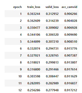
Go to the normal size

size = src_size
bs=3

data = (src
        .transform(get_transforms(), size=size, tfm_y=True)
        .databunch(bs=bs)
        .normalize(imagenet_stats))

learn = unet_learner(data, models.resnet34, metrics=metrics, wd=wd)
learn.load('stage-2');

lr_find(learn)
learn.recorder.plot()

1550783772526

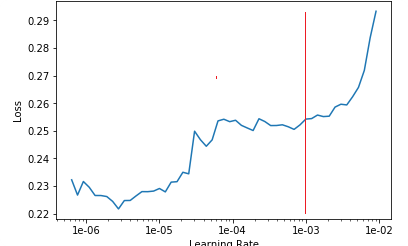
lr=1e-3
learn.fit_one_cycle(10, slice(lr), pct_start=0.8)

1550783798472

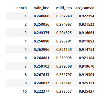
learn.unfreeze()
lrs = slice(1e-6,lr/10)
learn.fit_one_cycle(10, lrs)

learn.save('stage-2-big')

1550783824462

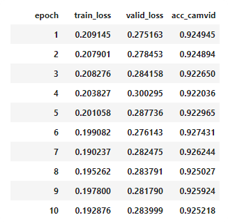
learn.load('stage-2-big');
learn.show_results(rows=3, figsize=(10,10))

1550783851169

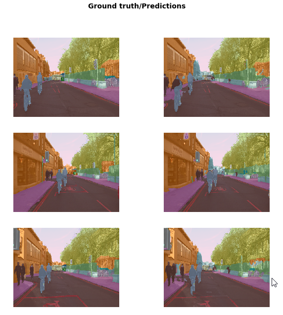
IMDB / NLP Text Classification

For text classification we can use IMDB database with reviews to check if review is positive or negative. We cannot use text directly in our fastai library. 1st we need tokenize the text and replace the text values with a number. For this we need to have vocabulary.

%reload_ext autoreload
%autoreload 2
%matplotlib inline

from fastai.text import *

bs = 48
path = untar_data(URLs.IMDB)
path.ls()

1551279684037

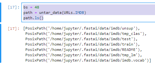
In the fastai library when you download your data, you’ve got your vocabulary in the dataset. (imdb.vocab), also you have your temporary language model that has labels equal 0 as (tmp_lm).

We load our Language Model Databunch. This is special DataBunch model without labels (labels are constant equal 0) . This data

data_lm = TextLMDataBunch.load(path, 'tmp_lm', bs=bs) #lm is a laguage model

# OR LONGER VERSION

# data_lm = (TextList.from_folder(path)
#            #Inputs: all the text files in path
#             .filter_by_folder(include=['train', 'test', 'unsup']) 
#            #We may have other temp folders that contain text files so we only keep what's in train and test
#             .random_split_by_pct(0.1)
#            #We randomly split and keep 10% (10,000 reviews) for validation
#             .label_for_lm()           
#            #We want to do a language model so we label accordingly (label = 0)
#             .databunch(bs=bs))

data_lm.show_batch()

1551281143436

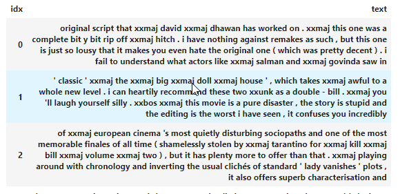
language_model_learner is used to predict next word in the sentence. AWD_LSTM is a model for text, that was pretrained on the english wikipedia. But the IMDB reviews contains language that is not the same as used in the wikipedia. That’s why we need to add a new vocabulary, and retrain the model with new text.

learn = language_model_learner(data_lm, AWD_LSTM, drop_mult=0.3)

learn.lr_find()
learn.recorder.plot(skip_end=15)

1551280626376

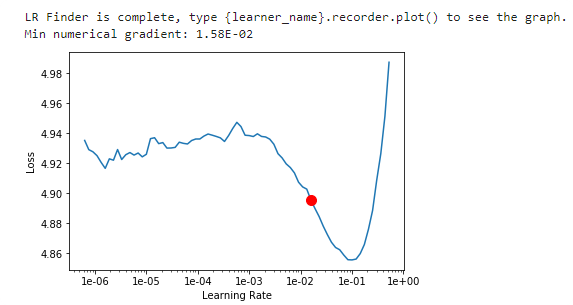
learn.fit_one_cycle(1, 1e-2, moms=(0.8,0.7))
learn.save('fit-01');

1551280644438

Accurracy is not great, but it is enough to train our model, but guessing next word is not an easy task even for huma.

learn.unfreeze()
learn.fit_one_cycle(10, 1e-3, moms=(0.8,0.7))

1551280679602

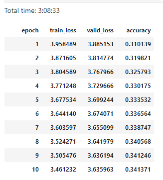
We save our model, and our encoder in the new file.

learn.save('fit-tuned')
learn.save_encoder('fit-tuned-enc')

We can test our encoder on some predefined text.

TEXT = "I liked this movie because"
N_WORDS = 40
N_SENTENCES = 2

learn.load('fit-tuned')
print("\n".join(learn.predict(TEXT, N_WORDS, temperature=0.75) for _ in range(N_SENTENCES)))

1551281719408

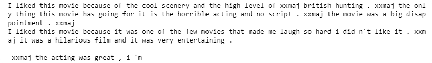
Next step is to use this learner as an encoder. This is now TextClasDataBunch, that try categorize our data.

path = untar_data(URLs.IMDB)

data_clas = TextClasDataBunch.load(path, 'tmp_clas', bs=bs)

# OR LONGER VERSION

# data_clas = (TextList.from_folder(path, vocab=data_lm.vocab)
#              #grab all the text files in path
#              .split_by_folder(valid='test')
#              #split by train and valid folder (that only keeps 'train' and 'test' so no need to filter)
#              .label_from_folder(classes=['neg', 'pos'])
#              #label them all with their folders
#              .databunch(bs=bs))

data_clas.show_batch()

1551281169972

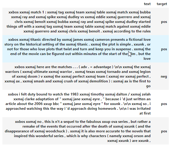
Now we create a text_classifier_learner, that is used for text classification, based on the same model AWD_LSTM. The only difference is that we also add load_encoder. Encoder is used in seq2seq more, by techinque called trasfer learning.

The encoder is essentially tasked with creating a mathematical representation of the language based on the task for predicting the next word.
A decoder is responsible for taking that representation and applying it to some problem (e.g., predicting the next word, understanding sentiment, etc…) source

We get our encoder that helps faster classify data, because it is used previously learned network.

learn = text_classifier_learner(data_clas, AWD_LSTM, drop_mult=0.5)
learn.load_encoder('fine_tuned_enc')

We freeze to last -3 layers.

learn.lr_find()
learn.recorder.plot()
learn.fit_one_cycle(1, slice(5e-3/(2.6**4),5e-3), moms=(0.8,0.7))

1551281849210

We now unfreeze our last two layers, and retrain a model.

learn.freeze_to(-2)
learn.fit_one_cycle(1, slice(1e-2/(2.6**4),1e-2), moms=(0.8,0.7))

1551281895175

learn.freeze_to(-3)
learn.fit_one_cycle(1, slice(5e-3/(2.6**4),5e-3), moms=(0.8,0.7))

1551281913865

learn.unfreeze()
learn.fit_one_cycle(2, slice(1e-3/(2.6**4),1e-3), moms=(0.8,0.7))

1551281930937

The last step is to predict on the example.

learn.predict("I really loved that movie, it was awesome!")

1551281976865

Twitter / Text recognition

On the webpage you can check working example on the current twitter statuses https://klemenko.pl/twitter.

1551282519719

I am using my own prepared data based on the EmoInt(Shared Task on Emotion Intesity) http://saifmohammad.com/WebPages/EmotionIntensity-SharedTask.html download . This data contains categorized text on real source. These emotions are [anger,fear,joy,sadness].

1551282811689

1551282849287

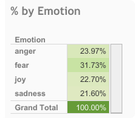
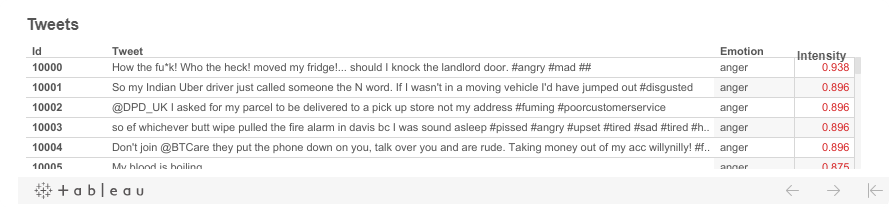
First we look to our data:

import numpy as np
import pandas as pd

import numpy as np
import pandas as pd

path = './textdata'
file = 'twitter.csv'

df = pd.read_csv(path + '/' + file)
df[:5]
df.groupby('Style').count()

1551282940905

1551282958641

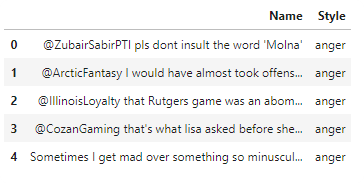
Because we don’t have vocabs, we need to create one, and save labels.

from fastai.text import *

data_lm = TextLMDataBunch.from_csv(path,file,text_cols='Name',label_cols='Style')
data_lm.save('labels')

We prepare learner like in the IMDB database.

learn = language_model_learner(data_lm, AWD_LSTM, drop_mult=0.3)
learn.lr_find()
learn.recorder.plot(skip_end=15)

1551283064635

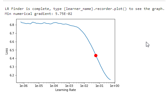
learn.fit_one_cycle(5, 1e-2)

1551283091608

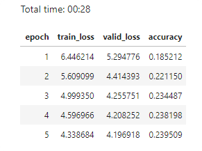
learn.unfreeze()
learn.fit_one_cycle(5, 1e-3, moms=(0.8,0.7))

1551283128284

learn.fit_one_cycle(20, 1e-2, moms=(0.8,0.7))

1551283164603

Now we save our model and encoder.

learn.save('fit-03')
learn.save_encoder('fine_tuned_enc')

Classifier

After we save our encoder, we can move to the classifier. When we load TextClasDataBunch, it is required to have vocab, for imdb it was already ther, but now, we can use TextLMDataBunch vocab loaded previously.

data_clas = TextClasDataBunch.from_csv(path,file,
                                       text_cols=text_col,
                                       label_cols=label_col,
                                       vocab=data_lm.vocab)

data_clas.show_batch()

1551283410731

We now create text classifier and learn to predict them emotions, using saved previously encoder.

learn = text_classifier_learner(data_clas, AWD_LSTM, drop_mult=0.5)
learn.load_encoder('fine_tuned_enc')

learn.lr_find()
learn.recorder.plot()

1551283502675

learn.fit_one_cycle(1, 1e-2)
learn.fit_one_cycle(10, 1e-2)
learn.save('text-01')

learn.freeze_to(-2)
learn.fit_one_cycle(1, slice(1e-2/(2.6**4),1e-2), moms=(0.8,0.7))


learn.fit_one_cycle(10, slice(1e-1/(2.6**4),1e-2), moms=(0.8,0.7))
learn.fit_one_cycle(20, slice(1e-1/(2.6**4),1e-2), moms=(0.8,0.7))

learn.fit_one_cycle(15, slice(1e-6,1e-6), moms=(0.8,0.7))

The first hit wasn’t so sucecsfull, but after a lot of training I end up with the 0.79 accuracy.

1551283588598

1551283639923

Now you can predict some text.

learn.predict("You are a lovely boy")

learn.predict("More evidence Trump relies on Putin's advice as much or more than US intelligence—a violation of his")

learn.save('text-02	')
learn.export()

1551283694281

1551283703083

Twitter Implementation

Install your twitter library.

!pip install python-twitter

For twitter you need to have a valid phone, with active account. On the webpage https://developer.twitter.com/en/apps, you can create a new app, and on the Keys and tokens you will have 4 values for your keys that you need to write in your project.

1551284072912

You can now write your

import twitter

api = twitter.Api(consumer_key='XXX',
                      consumer_secret='XXX',
                      access_token_key='XXX',
                      access_token_secret='XXX')

api.VerifyCredentials()

1551284213322

api.GetFriends()

1551284243248

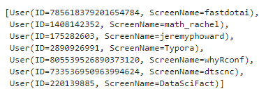
api.GetSearch('obama',count=30,lang='en')

1551284663961

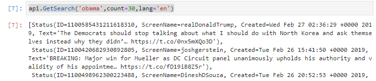
We can now define predictfunction, and get_tweetsfunction to return data.

from fastai.text import *
#learn_tweets = load_learner('textdata'); # !! YOUR FOLDER OF THE MODEL!!

def predict(text):
     return str(learn.predict(text)[0])

    
predict('some text')

1551284560815

def get_tweets(search):
    text = api.GetSearch(search,count=30,lang='en')
    textDict = [t.AsDict() for t in text]
    return [[predict(t['text']), t['text'], t['user']['screen_name']] for t in textDict]

get_tweets('obama')

1551284806471

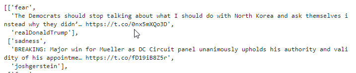
Tabular Data

For learning we can also use our DataFrame as a source, to predict values based on columns instead of images or text. This is categorization problem with we predict if the person ear less than 50k or more or equal 50,000 dolars, based on his status, occuppation etc...

from fastai.tabular import *

path = untar_data(URLs.ADULT_SAMPLE)
df = pd.read_csv(path/'adult.csv')

dep_var = 'salary'
cat_names = ['workclass', 'education', 'marital-status', 'occupation', 'relationship', 'race']
cont_names = ['age', 'fnlwgt', 'education-num']
procs = [FillMissing, Categorify, Normalize]

We prepare test data, and data to learn. We need define cat_names for categorical data, cont_names for number values, and procs to prepare our data before learn.

FillMissing - Fill missing Values
Categorify - Transform the categorical variables to that type.
Normalize - Normalize number values

We also add_test

test = TabularList.from_df(df.iloc[800:1000].copy(), 
                           path=path, 
                           cat_names=cat_names, 
                           cont_names=cont_names)

data = (TabularList.from_df(df, path=path, 
                            cat_names=cat_names, 
                            cont_names=cont_names, 
                            procs=procs)
                           .split_by_idx(list(range(800,1000)))
                           .label_from_df(cols=dep_var)
                           .add_test(test)
                           .databunch())

data.show_batch(rows=10)

1551285333505

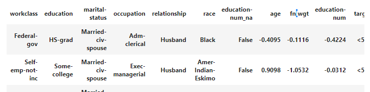
Now we prepare tabular_learner. We need specify matrices and layers. This will create two BatchNorm1D layers, one with the size 200, and one with the size 100, between each layer there is ReLU activation function, nad last is Linear layer.

learn = tabular_learner(data, layers=[200,100], metrics=accuracy)
learn.model

1551285643382

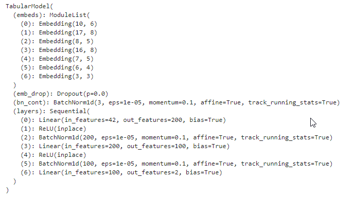
We can fit the value, and predict some value.

learn.fit(1, 1e-2)
row = df.iloc[0]
learn.predict(row)

1551285779712

1551285767498

Collaborative Matrix / Predict movie score for the user

If we have list of users and score for movies, we can show this as a 2D matrix (two dimensional tensor). When on rows we will have users, and on columns will have movies. Of course there is some missing points. Some users doesn’t set a score for a movie. That’s why we can fill missing values.

1551885030551

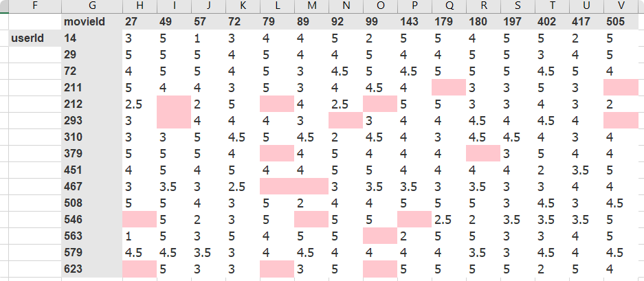
It can be done by Embedding matrices. As parameters (weigths as yellow cells and bias as blue cells), we can find a prediction for missing movie scores (orange cells). The width of the matrix is called n_factors - how big is the matrix to calculate result (in the example 4). On the output you can find missing values.

1551948571334

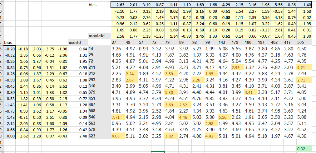
Implement in fast.ai

The data for movies can be downloaded from the MovieLens dataset: http://files.grouplens.org/datasets/movielens/ml-100k.zip. When we extract the data we found a lot of files. For our purpose we need only u.data that contain ratings, and u.item that contains titles for movies.

1551889081731

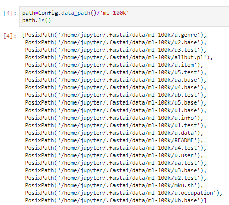
Becaise there is no header, and delimiter for csv is unusual a tab instead of semicolon, we need to define columns, and delimeer for data.

from fastai.collab import *
from fastai.tabular import *

path=Config.data_path()/'ml-100k'

user,item,title = 'userId','movieId','title'
ratings = pd.read_csv(path/'u.data', 
                      delimiter='\t', 
                      header=None,
                      names=[user, item,'rating','timestamp'])

ratings.head()

1551889251429

movies = pd.read_csv(path/'u.item',  
                     delimiter='|', 
                     encoding='latin-1',
                     header=None,
                     names=[item, 'title', 'date', 'N', 'url', *[f'g{i}' for i in range(19)]])
movies.head()

delimiter now is |, and encoding is latin-2, because there are also 19 columns that is not important for us (the genre of the movie), we define them as a list of g* columns
*[f'g{i}' for i in range(19)] - star * means that we don’t add the array but values of the array to the array names

1551889563326

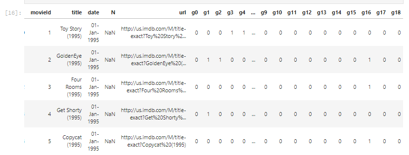
We can now combine ratings and movies. This is done by column movieId

rating_movie = ratings.merge(movies[[item, title]])
rating_movie.head()

1551889619310

We can now create DataBunch for movies, and users.

seed -parameter for split_by_random_pct, seed value for generate random values
pct_val - number of validation set
item_name - name show in the output batch.

data = CollabDataBunch.from_df(rating_movie, 
                               seed=42, 
                               valid_pct=0.1,  #changed in the new version
                               item_name=title)
data.show_batch()

1551889983434

Now we can create collab_learner for collaborative matrix.

n_factors - size of the embedding matrix
y_range - range of the score. It is better to setup little more than maximum (5.5), because in the sigmoid activation the output never touch maximum value, and sometimes it happens that user score a movie as a 5.

y_range = [0,5.5]

learn = collab_learner(data, n_factors=40, y_range=y_range, wd=1e-1)
learn.model

learn.lr_find()
learn.recorder.plot(skip_end=15)

1551890251264

1551890204073

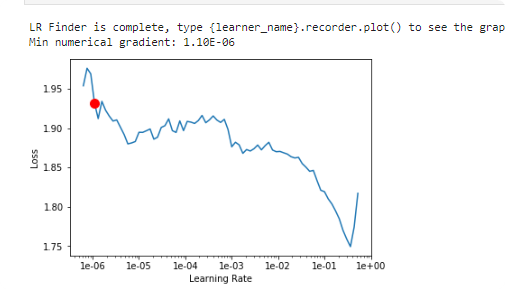
We now fit our model

learn.fit_one_cycle(5, 5e-3)
learn.save('dotprod')

1551890223039

Predict

You can now predict your model based on userId and title:

learn.predict({'userId': 196, 'title': 'Philadelphia (1993)'	})

If you got error: RuntimeError: Expected object of backend CPU but got backend CUDA for argument #3 'index', just put learn.model.cuda() before predict.

1554545660312

learn.model.cuda()
learn.predict({'userId': 196, 'title': 'Philadelphia (1993)'})

1554545743870

Bias

Bias for movie can define the total score. Let’s

define the top 1000 movies by the score.

g = rating_movie.groupby(title)['rating'].count() 
top_movies = g.sort_values(ascending=False).index.values[:1000]

1551890952660

Get bias for each movie in the array. is_item means that it will be looking by the item name instead of user id. mean_ratings are real values for ratings, and movie_ratings are ratings defined from the movie_bias array.

movie_bias = learn.bias(top_movies, is_item=True)
mean_ratings = rating_movie.groupby(title)['rating'].mean()
movie_ratings = [(b, i, mean_ratings.loc[i]) for i,b in zip(top_movies,movie_bias)]

sorted(movie_ratings, key=lambda o: o[0], reverse=True)[:15]

1551891196592

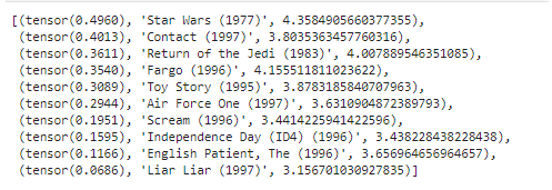
The result is similar to the real values, but this is unbiased value of how movie is good.
user bias we can interpret as overall how this user rate movies

movie bias numbers as a way of saying what are the best movies or what do people really like as movies even if those people don't rate movies very highly or even if that movie doesn't have the kind of features that people tend to rate highly. (jeremy howard)

Movie weights

We can get weights and squeeze them into 3 factors, by using pca.This will reduce number of columns

movie_w = learn.weight(top_movies, is_item=True)
movie_pca = movie_w.pca(3)
fac0,fac1,fac2 = movie_pca.t()

pca can define hidden meaning of weights and define a 3 different approches that is get to the output.
fac0 - define the one factor on movies that on top are classic movies, and on the bottom are also popular movies, but not defined as a classic one. We can call this division as a connoisseur level

movies_fac0 = [(f, i) for f,i in zip(fac0, top_movies)]
[ 
    *sorted(movies_fac0, key=itemgetter(0), reverse=True)[:10],
    *sorted(movies_fac0, key=itemgetter(0))[:10]
]

1551892475753

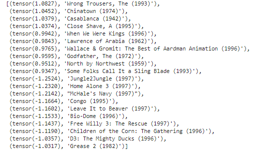
fac1 - We can define them as a great hits on the top, and on bottom some disutopian movies or more brutal that are not for everewhyone.

movies_fac1 = [(f, i) for f,i in zip(fac1, top_movies)]
[ 
    *sorted(movies_fac1, key=itemgetter(0), reverse=True)[:10],
    *sorted(movies_fac1, key=itemgetter(0))[:10]
]

1551892653296

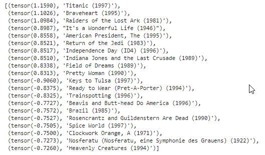
fac2 0 The same for

movies_fac2 = [(f, i) for f,i in zip(fac2, top_movies)]
[ 
    *sorted(movies_fac2, key=itemgetter(0), reverse=True)[:10],
    *sorted(movies_fac2, key=itemgetter(0))[:10]
]

1551893011316

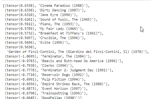
We can plot pca fac0 and fac2 together on one plot. (the color is random)

idxs = np.random.choice(len(top_movies), 50, replace=False)
idxs = list(range(50))
X = fac0[idxs]
Y = fac2[idxs]

plt.figure(figsize=(15,15))
plt.scatter(X, Y)

for  i, x, y,c in zip(top_movies[idxs], X, Y,Z):
    plt.text(x,y,i, color=np.random.rand(3)*0.7*0.7, fontsize=11)
plt.show()

1551893767396

# GPU Servers

# Artificial Neural Network more

# Single Layer Perceptron

# When Use?

# Modern Neural Network

# Forward Function

# Gradient Descent more

# Backpropagation

# Pytorch Implementation

# Do I have to implement all these functions?

# Using Sequential

# Using nn.Model

# Example of SGD for linear function

# Data / Source

# Resources

# Text Resources:

# Tabular Data

# Data Download / Google Drive

# Data Download / Google Images

# Data Download / wget

# Data Download / kaggle

# Data Download / linux commands

# Architecture

# Glossary

# Activation Functions more

# Sigmoid function

# When Use?

# List of Activation functions source

# When Use?

# Loss functions more PyTorch

# weight decay - SGD - L2 Regularization

# Momentum more

# RMSProp

# Adam Optimizer

# Convolution Network more

# F.conv2d

# stride

# padding

# nn.Conv2d

# The size of the output more

# Examples:

# NETRON

# Batch Normalization more paper video

# Dropout paper video

# PyTorch WebPage

# Functions

# How to train a model?

# DataSet / DataLoader

# Model

# Backward propagation

# Learn

# Using 2 layer model

# Adam optimizer

# Using model with fastai

# fast.ai github

# Installation / Google Colab source

# installion / AWS

# installation / Google Cloud

# fast.ai / Help functions

# open_image()

# open_mask(fn)

# .show()

# .apply_tfms()

# ImageCleaner

# .show_heatmap()

# Another layer

# fast.ai / Data

# Basic functions

# ImageDataBunch

# ImageDataBunch / from_folder

# ImageDataBunch / from_csv

# ImageDataBunch / from_df

# ImageDataBunch / from_name_re

# ImageDataBunch / from_name_func

# ImageDataBunch / from_list

# DataBunch / Own Item List

# Examples 1/ Planet Data

# Example 2 / IMDB DataBase

# DataBunch / 1. DataType more

# DataBunch / 2. from_

GPU Servers

Artificial Neural Network more

Single Layer Perceptron

When Use?

Modern Neural Network

Forward Function

Gradient Descent more

Backpropagation

Pytorch Implementation

Do I have to implement all these functions?

Using Sequential

Using nn.Model

Example of SGD for linear function

Data / Source

Resources

Text Resources:

Tabular Data

Data Download / Google Drive

Data Download / Google Images

Data Download / wget

Data Download / kaggle

Data Download / linux commands

Architecture

Glossary

Activation Functions more

Sigmoid function

When Use?

List of Activation functions source

When Use?

Loss functions more PyTorch

weight decay - SGD - L2 Regularization

Momentum more

RMSProp

Adam Optimizer

Convolution Network more

F.conv2d

stride

padding

nn.Conv2d

The size of the output more

Examples:

NETRON

Batch Normalization more paper video

Dropout paper video

PyTorch WebPage

Functions

How to train a model?

DataSet / DataLoader

Model

Backward propagation

Learn

Using 2 layer model

Adam optimizer

Using model with fastai

fast.ai github

Installation / Google Colab source

installion / AWS

installation / Google Cloud

fast.ai / Help functions

open_image()

open_mask(fn)

.show()

.apply_tfms()

ImageCleaner

.show_heatmap()

Another layer

fast.ai / Data

Basic functions

ImageDataBunch

ImageDataBunch / from_folder

ImageDataBunch / from_csv

ImageDataBunch / from_df

ImageDataBunch / from_name_re

ImageDataBunch / from_name_func

ImageDataBunch / from_list

DataBunch / Own Item List

Examples 1/ Planet Data

Example 2 / IMDB DataBase

DataBunch / 1. DataType more

DataBunch / 2. from_